Regional Tropical Precipitation Change ... - Academia Sinica

More documents

Recommendations

Info

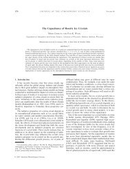
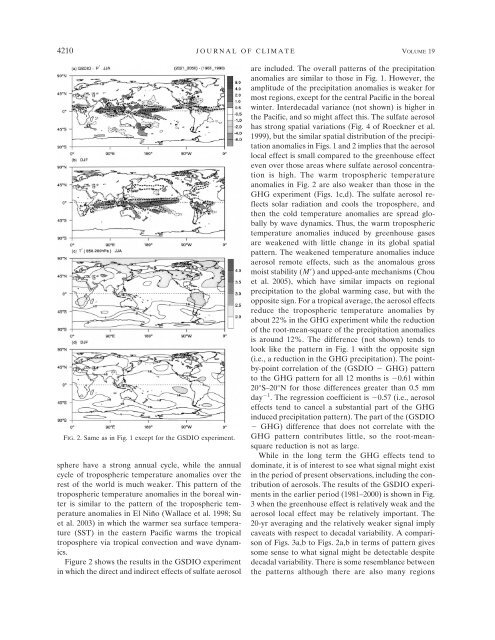
4210 JOURNAL OF CLIMATE VOLUME 19 FIG. 2. Same as in Fig. 1 except for the GSDIO experiment. sphere have a strong annual cycle, while the annual cycle of tropospheric temperature anomalies over the rest of the world is much weaker. This pattern of the tropospheric temperature anomalies in the boreal winter is similar to the pattern of the tropospheric temperature anomalies in El Niño (Wallace et al. 1998; Su et al. 2003) in which the warmer sea surface temperature (SST) in the eastern Pacific warms the tropical troposphere via tropical convection and wave dynamics. Figure 2 shows the results in the GSDIO experiment in which the direct and indirect effects of sulfate aerosol are included. The overall patterns of the precipitation anomalies are similar to those in Fig. 1. However, the amplitude of the precipitation anomalies is weaker for most regions, except for the central Pacific in the boreal winter. Interdecadal variance (not shown) is higher in the Pacific, and so might affect this. The sulfate aerosol has strong spatial variations (Fig. 4 of Roeckner et al. 1999), but the similar spatial distribution of the precipitation anomalies in Figs. 1 and 2 implies that the aerosol local effect is small compared to the greenhouse effect even over those areas where sulfate aerosol concentration is high. The warm tropospheric temperature anomalies in Fig. 2 are also weaker than those in the GHG experiment (Figs. 1c,d). The sulfate aerosol reflects solar radiation and cools the troposphere, and then the cold temperature anomalies are spread globally by wave dynamics. Thus, the warm tropospheric temperature anomalies induced by greenhouse gases are weakened with little change in its global spatial pattern. The weakened temperature anomalies induce aerosol remote effects, such as the anomalous gross moist stability (M) and upped-ante mechanisms (Chou et al. 2005), which have similar impacts on regional precipitation to the global warming case, but with the opposite sign. For a tropical average, the aerosol effects reduce the tropospheric temperature anomalies by about 22% in the GHG experiment while the reduction of the root-mean-square of the precipitation anomalies is around 12%. The difference (not shown) tends to look like the pattern in Fig. 1 with the opposite sign (i.e., a reduction in the GHG precipitation). The pointby-point correlation of the (GSDIO GHG) pattern to the GHG pattern for all 12 months is 0.61 within 20°S–20°N for those differences greater than 0.5 mm day 1 . The regression coefficient is 0.57 (i.e., aerosol effects tend to cancel a substantial part of the GHG induced precipitation pattern). The part of the (GSDIO GHG) difference that does not correlate with the GHG pattern contributes little, so the root-meansquare reduction is not as large. While in the long term the GHG effects tend to dominate, it is of interest to see what signal might exist in the period of present observations, including the contribution of aerosols. The results of the GSDIO experiments in the earlier period (1981–2000) is shown in Fig. 3 when the greenhouse effect is relatively weak and the aerosol local effect may be relatively important. The 20-yr averaging and the relatively weaker signal imply caveats with respect to decadal variability. A comparison of Figs. 3a,b to Figs. 2a,b in terms of pattern gives some sense to what signal might be detectable despite decadal variability. There is some resemblance between the patterns although there are also many regions
1SEPTEMBER 2006 C H O U E T A L . 4211 FIG. 3. <strong>Precipitation</strong> differences (mm day 1 ) between the 1981– 2000 and 1961–80 averages for the GSDIO experiment in (a) JJA and (b) DJF. where substantial differences occur due to decadal variability. This suggests that it may be challenging to infer the long-term GHG effect reliably from recent observed trends, except for particular regions such as eastern South America in DJF and the Caribbean in JJA. 4. Atmospheric versus oceanic feedbacks To understand the oceanic feedbacks, we compare experiments with the ECHAM4 atmospheric model coupled with an ML ocean, with normal and doubled carbon dioxide concentrations, respectively. This pair of experiments with no ocean feedback (Fig. 5) is compared to the GHG experiment with differences between 1961–90 and 2070–99 (Fig. 4) when carbon dioxide concentration is roughly doubled. Note that besides the difference in oceanic feedback, the ML experiments are an equilibrium simulation, but the GHG experiment is a transient simulation. For the longer GHG simulation shown in Fig. 4, the spatial distributions of the precipitation and tropospheric temperature anomalies are very similar to the anomalies in the earlier period shown in Fig. 1, but with stronger amplitude. This implies that the changes in temperature and precipitation induced by the greenhouse effect are already established in 2021–50 and the patterns tend to grow and persist over the century. Most tropical precipitation anomalies in the ML experiments (Fig. 5) are similar to those in the GHG experiment when ocean dynamical FIG. 4. Same as in Fig. 1 except for differences between 2070–99 and 1961–90. feedback is included (Fig. 4), except for the Pacific. In the Pacific, oceanic feedback tends to shift the positive precipitation anomalies eastward. Without oceanic feedback, almost all positive precipitation anomalies in the Tropics occur over convective regions, while the negative precipitation anomalies occur over margins of convective regions [e.g., South America and the Indian Ocean in DJF (the boxes in Fig. 5b)]. This distribution of the regional tropical precipitation anomalies (Fig. 5) is very similar to those found in CN04. In their study, they also used an ML ocean without considering ocean
Page 1 and 2: 1SEPTEMBER 2006 C H O U E T A L . 4
Page 3: 1SEPTEMBER 2006 C H O U E T A L . 4
Page 17: 1SEPTEMBER 2006 C H O U E T A L . 4

Regional Tropical Precipitation Change ... - Academia Sinica

Create successful ePaper yourself

Delete template?

Save as template?