EXAMPLES: MIXTURE MODELING WITH CROSS ... - Mplus

Examples: Mixture Modeling With Cross-Sectional Data 

CHAPTER 7 

EXAMPLES: MIXTURE 

MODELING WITH CROSS- 

SECTIONAL DATA 

Mixture modeling refers to modeling with categorical latent variables 

that represent subpopulations where population membership is not 

known but is inferred from the data. This is referred to as finite mixture 

modeling in statistics (McLachlan & Peel, 2000). A special case is 

latent class analysis (LCA) where the latent classes explain the 

relationships among the observed dependent variables similar to factor 

analysis. In contrast to factor analysis, however, LCA provides 

classification of individuals. In addition to conventional exploratory 

LCA, confirmatory LCA and LCA with multiple categorical latent 

variables can be estimated. In Mplus, mixture modeling can be applied 

to any of the analyses discussed in the other example chapters including 

regression analysis, path analysis, confirmatory factor analysis (CFA), 

item response theory (IRT) analysis, structural equation modeling 

(SEM), growth modeling, survival analysis, and multilevel modeling. 

Observed dependent variables can be continuous, censored, binary, 

ordered categorical (ordinal), unordered categorical (nominal), counts, 

or combinations of these variable types. LCA and general mixture 

models can be extended to include continuous latent variables. An 

overview can be found in Muthén (2008). 

LCA is a measurement model. A general mixture model has two parts: a 

measurement model and a structural model. The measurement model for 

LCA and the general mixture model is a multivariate regression model 

that describes the relationships between a set of observed dependent 

variables and a set of categorical latent variables. The observed 

dependent variables are referred to as latent class indicators. The 

relationships are described by a set of linear regression equations for 

continuous latent class indicators, a set of censored normal or censoredinflated 

normal regression equations for censored latent class indicators, 

a set of logistic regression equations for binary or ordered categorical 

latent class indicators, a set of multinomial logistic regressions for 

unordered categorical latent class indicators, and a set of Poisson or 

153

CHAPTER 7 

zero-inflated Poisson regression equations for count latent class 

indicators. 

The structural model describes three types of relationships in one set of 

multivariate regression equations: the relationships among the 

categorical latent variables, the relationships among observed variables, 

and the relationships between the categorical latent variables and 

observed variables that are not latent class indicators. These 

relationships are described by a set of multinomial logistic regression 

equations for the categorical latent dependent variables and unordered 

observed dependent variables, a set of linear regression equations for 

continuous observed dependent variables, a set of censored normal or 

censored normal regression equations for censored-inflated observed 

dependent variables, a set of logistic regression equations for binary or 

ordered categorical observed dependent variables, and a set of Poisson 

or zero-inflated Poisson regression equations for count observed 

dependent variables. For logistic regression, ordered categorical 

variables are modeled using the proportional odds specification. 

Maximum likelihood estimation is used. 

The general mixture model can be extended to include continuous latent 

variables. The measurement and structural models for continuous latent 

variables are described in Chapter 5. In the extended general mixture 

model, relationships between categorical and continuous latent variables 

are allowed. These relationships are described by a set of multinomial 

logistic regression equations for the categorical latent dependent 

variables and a set of linear regression equations for the continuous 

latent dependent variables. 

In mixture modeling, some starting values may result in local solutions 

that do not represent the global maximum of the likelihood. To avoid 

this, different sets of starting values are automatically produced and the 

solution with the best likelihood is reported. 

All cross-sectional mixture models can be estimated using the following 

special features: 

• Single or multiple group analysis 

• Missing data 

• Complex survey data 

154


• Latent variable interactions and non-linear factor analysis using 

maximum likelihood 

• Random slopes 

• Linear and non-linear parameter constraints 

• Indirect effects including specific paths 

• Maximum likelihood estimation for all outcome types 

• Bootstrap standard errors and confidence intervals 

• Wald chi-square test of parameter equalities 

• Test of equality of means across latent classes using posterior 

probability-based multiple imputations 

For TYPE=MIXTURE, multiple group analysis is specified by using the 

KNOWNCLASS option of the VARIABLE command. The default is to 

estimate the model under missing data theory using all available data. 

The LISTWISE option of the DATA command can be used to delete all 

observations from the analysis that have missing values on one or more 

of the analysis variables. Corrections to the standard errors and chisquare 

test of model fit that take into account stratification, nonindependence 

of observations, and unequal probability of selection are 

obtained by using the TYPE=COMPLEX option of the ANALYSIS 

command in conjunction with the STRATIFICATION, CLUSTER, and 

WEIGHT options of the VARIABLE command. The 

SUBPOPULATION option is used to select observations for an analysis 

when a subpopulation (domain) is analyzed. Latent variable interactions 

are specified by using the | symbol of the MODEL command in 

conjunction with the XWITH option of the MODEL command. Random 

slopes are specified by using the | symbol of the MODEL command in 

conjunction with the ON option of the MODEL command. Linear and 

non-linear parameter constraints are specified by using the MODEL 

CONSTRAINT command. Indirect effects are specified by using the 

MODEL INDIRECT command. Maximum likelihood estimation is 

specified by using the ESTIMATOR option of the ANALYSIS 

command. Bootstrap standard errors are obtained by using the 

BOOTSTRAP option of the ANALYSIS command. Bootstrap 

confidence intervals are obtained by using the BOOTSTRAP option of 

the ANALYSIS command in conjunction with the CINTERVAL option 

of the OUTPUT command. The MODEL TEST command is used to test 

linear restrictions on the parameters in the MODEL and MODEL 

CONSTRAINT commands using the Wald chi-square test. The 

AUXILIARY option is used to test the equality of means across latent 

classes using posterior probability-based multiple imputations. 

155

CHAPTER 7 

Graphical displays of observed data and analysis results can be obtained 

using the PLOT command in conjunction with a post-processing 

graphics module. The PLOT command provides histograms, 

scatterplots, plots of individual observed and estimated values, plots of 

sample and estimated means and proportions/probabilities, and plots of 

estimated probabilities for a categorical latent variable as a function of 

its covariates. These are available for the total sample, by group, by 

class, and adjusted for covariates. The PLOT command includes 

a display showing a set of descriptive statistics for each variable. The 

graphical displays can be edited and exported as a DIB, EMF, or JPEG 

file. In addition, the data for each graphical display can be saved in an 

external file for use by another graphics program. 

Following is the set of examples included in this chapter. 

• 7.1: Mixture regression analysis for a continuous dependent 

variable using automatic starting values with random starts 

• 7.2: Mixture regression analysis for a count variable using a zeroinflated 

Poisson model using automatic starting values with random 

starts 

• 7.3: LCA with binary latent class indicators using automatic starting 

values with random starts 

• 7.4: LCA with binary latent class indicators using user-specified 

starting values without random starts 

• 7.5: LCA with binary latent class indicators using user-specified 

starting values with random starts 

• 7.6: LCA with three-category latent class indicators using userspecified 


• 7.7: LCA with unordered categorical latent class indicators using 

automatic starting values with random starts 

• 7.8: LCA with unordered categorical latent class indicators using 

user-specified starting values with random starts 

• 7.9: LCA with continuous latent class indicators using automatic 


• 7.10: LCA with continuous latent class indicators using userspecified 


• 7.11: LCA with binary, censored, unordered, and count latent class 

indicators using user-specified starting values without random starts 

• 7.12: LCA with binary latent class indicators using automatic 

starting values with random starts with a covariate and a direct effect 

156


• 7.13: Confirmatory LCA with binary latent class indicators and 

parameter constraints 

• 7.14: Confirmatory LCA with two categorical latent variables 

• 7.15: Loglinear model for a three-way table with conditional 

independence between the first two variables 

• 7.16: LCA with partial conditional independence* 

• 7.17: Mixture CFA modeling 

• 7.18: LCA with a second-order factor (twin analysis)* 

• 7.19: SEM with a categorical latent variable regressed on a 

continuous latent variable* 

• 7.20: Structural equation mixture modeling 

• 7.21: Mixture modeling with known classes (multiple group 

analysis) 

• 7.22: Mixture modeling with continuous variables that correlate 

within class 

• 7.23: Mixture randomized trials modeling using CACE estimation 

with training data 

• 7.24: Mixture randomized trials modeling using CACE estimation 

with missing data on the latent class indicator 

• 7.25: Zero-inflated Poisson regression carried out as a two-class 

model 

• 7.26: CFA with a non-parametric representation of a non-normal 

factor distribution 

• 7.27: Factor (IRT) mixture analysis with binary latent class and 

factor indicators* 

• 7.28: Two-group twin model for categorical outcomes using 

maximum likelihood and parameter constraints* 

• 7.29: Two-group IRT twin model for factors with categorical factor 

indicators using parameter constraints* 

• 7.30: Continuous-time survival analysis using a Cox regression 

model to estimate a treatment effect 

* Example uses numerical integration in the estimation of the model. 

This can be computationally demanding depending on the size of the 

problem. 

157

CHAPTER 7 

EXAMPLE 7.1: MIXTURE REGRESSION ANALYSIS FOR A 

CONTINUOUS DEPENDENT VARIABLE USING AUTOMATIC 

STARTING VALUES WITH RANDOM STARTS 

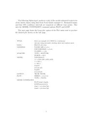
TITLE: this is an example of a mixture regression 

analysis for a continuous dependent 

variable using automatic starting values 

with random starts 

DATA: FILE IS ex7.1.dat; 

VARIABLE: NAMES ARE y x1 x2; 

CLASSES = c (2); 

ANALYSIS: TYPE = MIXTURE; 

MODEL: 

%OVERALL% 

y ON x1 x2; 

c ON x1; 

%c#2% 

y ON x2; 

y; 

OUTPUT: TECH1 TECH8; 

y 

c 

x1 

x2 

158


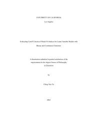
In this example, the mixture regression model for a continuous 

dependent variable shown in the picture above is estimated using 

automatic starting values with random starts. Because c is a categorical 

latent variable, the interpretation of the picture is not the same as for 

models with continuous latent variables. The arrow from c to y indicates 

that the intercept of y varies across the classes of c. This corresponds to 

the regression of y on a set of dummy variables representing the 

categories of c. The broken arrow from c to the arrow from x2 to y 

indicates that the slope in the regression of y on x2 varies across the 

classes of c. The arrow from x1 to c represents the multinomial logistic 

regression of c on x1. 

TITLE: 

this is an example of a mixture regression 

analysis for a continuous dependent 

variable 

The TITLE command is used to provide a title for the analysis. The title 

is printed in the output just before the Summary of Analysis. 

DATA: 

FILE IS ex7.1.dat; 

The DATA command is used to provide information about the data set 

to be analyzed. The FILE option is used to specify the name of the file 

that contains the data to be analyzed, ex7.1.dat. Because the data set is 

in free format, the default, a FORMAT statement is not required. 

VARIABLE: NAMES ARE y x1 x2; 


The VARIABLE command is used to provide information about the 

variables in the data set to be analyzed. The NAMES option is used to 

assign names to the variables in the data set. The data set in this 

example contains three variables: y, x1, and x2. The CLASSES option 

is used to assign names to the categorical latent variables in the model 

and to specify the number of latent classes in the model for each 

categorical latent variable. In the example above, there is one 

categorical latent variable c that has two latent classes. 

ANALYSIS: 

TYPE = MIXTURE; 

The ANALYSIS command is used to describe the technical details of the 

analysis. The TYPE option is used to describe the type of analysis that 

159

CHAPTER 7 

is to be performed. By selecting MIXTURE, a mixture model will be 

estimated. 

When TYPE=MIXTURE is specified, either user-specified or automatic 

starting values are used to create randomly perturbed sets of starting 

values for all parameters in the model except variances and covariances. 

In this example, the random perturbations are based on automatic 

starting values. Maximum likelihood optimization is done in two stages. 

In the initial stage, 20 random sets of starting values are generated. An 

optimization is carried out for ten iterations using each of the 20 random 

sets of starting values. The ending values from the 4 optimizations with 

the highest loglikelihoods are used as the starting values in the final 

stage optimizations which are carried out using the default optimization 

settings for TYPE=MIXTURE. A more thorough investigation of 

multiple solutions can be carried out using the STARTS and 

STITERATIONS options of the ANALYSIS command. 

MODEL: 

%OVERALL% 

y ON x1 x2; 

c ON x1; 

%c#2% 

y ON x2; 

y; 

The MODEL command is used to describe the model to be estimated. 

For mixture models, there is an overall model designated by the label 

%OVERALL%. The overall model describes the part of the model that 

is in common for all latent classes. The part of the model that differs for 

each class is specified by a label that consists of the categorical latent 

variable followed by the number sign followed by the class number. In 

the example above, the label %c#2% refers to the part of the model for 

class 2 that differs from the overall model. 

In the overall model, the first ON statement describes the linear 

regression of y on the covariates x1 and x2. The second ON statement 

describes the multinomial logistic regression of the categorical latent 

variable c on the covariate x1 when comparing class 1 to class 2. The 

intercept in the regression of c on x1 is estimated as the default. 

In the model for class 2, the ON statement describes the linear regression 

of y on the covariate x2. This specification relaxes the default equality 

160


constraint for the regression coefficient. By mentioning the residual 

variance of y, it is not held equal across classes. The intercepts in class 

1 and class 2 are free and unequal as the default. The default estimator 

for this type of analysis is maximum likelihood with robust standard 

errors. The ESTIMATOR option of the ANALYSIS command can be 

used to select a different estimator. 

Following is an alternative specification of the multinomial logistic 

regression of c on the covariate x1: 

c#1 ON x1; 

where c#1 refers to the first class of c. The classes of a categorical latent 

variable are referred to by adding to the name of the categorical latent 

variable the number sign (#) followed by the number of the class. This 

alternative specification allows individual parameters to be referred to in 

the MODEL command for the purpose of giving starting values or 

placing restrictions. 

OUTPUT: 

TECH1 TECH8; 

The OUTPUT command is used to request additional output not 

included as the default. The TECH1 option is used to request the arrays 

containing parameter specifications and starting values for all free 

parameters in the model. The TECH8 option is used to request that the 

optimization history in estimating the model be printed in the output. 

TECH8 is printed to the screen during the computations as the default. 

TECH8 screen printing is useful for determining how long the analysis 

takes. 

161

CHAPTER 7 

EXAMPLE 7.2: MIXTURE REGRESSION ANALYSIS FOR A 

COUNT VARIABLE USING A ZERO-INFLATED POISSON 

MODEL USING AUTOMATIC STARTING VALUES WITH 

RANDOM STARTS 

TITLE: this is an example of a mixture regression 

analysis for a count variable using a 

zero-inflated Poisson model using 

automatic starting values with random 

starts 


VARIABLE: NAMES ARE u x1 x2; 


COUNT = u (i); 


MODEL: 

%OVERALL% 

u ON x1 x2; 

u#1 ON x1 x2; 

c ON x1; 

%c#2% 

u ON x2; 


The difference between this example and Example 7.1 is that the 

dependent variable is a count variable instead of a continuous variable. 

The COUNT option is used to specify which dependent variables are 

treated as count variables in the model and its estimation and whether a 

Poisson or zero-inflated Poisson model will be estimated. In the 

example above, u is a count variable. The i in parentheses following u 

indicates that a zero-inflated Poisson model will be estimated. 

With a zero-inflated Poisson model, two regressions are estimated. In 

the overall model, the first ON statement describes the Poisson 

regression of the count part of u on the covariates x1 and x2. This 

regression predicts the value of the count dependent variable for 

individuals who are able to assume values of zero and above. The 

second ON statement describes the logistic regression of the binary 

latent inflation variable u#1 on the covariates x1 and x2. This 

regression describes the probability of being unable to assume any value 

except zero. The inflation variable is referred to by adding to the name 

of the count variable the number sign (#) followed by the number 1. The 

162


third ON statement specifies the multinomial logistic regression of the 

categorical latent variable c on the covariate x1 when comparing class 1 

to class 2. The intercept in the regression of c on x1 is estimated as the 

default. 

In the model for class 2, the ON statement describes the Poisson 

regression of the count part of u on the covariate x2. This specification 

relaxes the default equality constraint for the regression coefficient. The 

intercepts of u are free and unequal across classes as the default. All 

other parameters are held equal across classes as the default. The 

default estimator for this type of analysis is maximum likelihood with 

robust standard errors. The ESTIMATOR option of the ANALYSIS 

command can be used to select a different estimator. An explanation of 

the other commands can be found in Example 7.1. 

EXAMPLE 7.3: LCA WITH BINARY LATENT CLASS 

INDICATORS USING AUTOMATIC STARTING VALUES 

WITH RANDOM STARTS 

TITLE: 

this is an example of a LCA with binary 

latent class indicators using automatic 



VARIABLE: NAMES ARE u1-u4 x1-x10; 

USEVARIABLES = u1-u4; 


CATEGORICAL = u1-u4; 

AUXILIARY = x1-x10 (R3STEP); 


OUTPUT: TECH1 TECH8 TECH10; 

163

CHAPTER 7 

u1 

u2 

c 

u3 

u4 

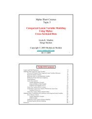
In this example, the latent class analysis (LCA) model with binary latent 

class indicators shown in the picture above is estimated using automatic 

starting values and random starts. Because c is a categorical latent 

variable, the interpretation of the picture is not the same as for models 

with continuous latent variables. The arrows from c to the latent class 

indicators u1, u2, u3, and u4 indicate that the thresholds of the latent 

class indicators vary across the classes of c. This implies that the 

probabilities of the latent class indicators vary across the classes of c. 

The arrows correspond to the regressions of the latent class indicators on 

a set of dummy variables representing the categories of c. 

The CATEGORICAL option is used to specify which dependent 

variables are treated as binary or ordered categorical (ordinal) variables 

in the model and its estimation. In the example above, the latent class 

indicators u1, u2, u3, and u4, are binary or ordered categorical variables. 

The program determines the number of categories for each indicator. 

The AUXILIARY option is used to specify variables that are not part of 

the analysis that are important predictors of latent classes using a threestep 

approach (Vermunt, 2010; Asparouhov & Muthén, 2012b). The 

letters R3STEP in parentheses is placed behind the variables in the 

AUXILIARY statement that that will be used as covariates in the third 

step multinomial logistic regression in a mixture model. 

164


The MODEL command does not need to be specified when automatic 

starting values are used. The thresholds of the observed variables and 

the mean of the categorical latent variable are estimated as the default. 

The thresholds are not held equal across classes as the default. The 



command can be used to select a different estimator. 

The TECH10 option is used to request univariate, bivariate, and 

response pattern model fit information for the categorical dependent 

variables in the model. This includes observed and estimated (expected) 

frequencies and standardized residuals. An explanation of the other 

commands can be found in Example 7.1. 


INDICATORS USING USER-SPECIFIED STARTING VALUES 

WITHOUT RANDOM STARTS 

TITLE: this is an example of a LCA with binary 

latent class indicators using userspecified 

starting values without random 

starts 


VARIABLE: NAMES ARE u1-u4; 




STARTS = 0; 

MODEL: 

%OVERALL% 

%c#1% 

[u1$1*1 u2$1*1 u3$1*-1 u4$1*-1]; 

%c#2% 

[u1$1*-1 u2$1*-1 u3$1*1 u4$1*1]; 


The differences between this example and Example 7.3 are that userspecified 

starting values are used instead of automatic starting values 

and there are no random starts. By specifying STARTS=0 in the 

ANALYSIS command, random starts are turned off. 

165

CHAPTER 7 

In the MODEL command, user-specified starting values are given for the 

thresholds of the binary latent class indicators. For binary and ordered 

categorical dependent variables, thresholds are referred to by adding to a 

variable name a dollar sign ($) followed by a threshold number. The 

number of thresholds is equal to the number of categories minus one. 

Because the latent class indicators are binary, they have one threshold. 

The thresholds of the latent class indicators are referred to as u1$1, 

u2$1, u3$1, and u4$1. Square brackets are used to specify starting 

values in the logit scale for the thresholds of the binary latent class 

indicators. The asterisk (*) is used to assign a starting value. It is placed 

after a variable with the starting value following it. In the example 

above, the threshold of u1 is assigned the starting value of 1 for class 1 

and -1 for class 2. The threshold of u4 is assigned the starting value of - 

1 for class 1 and 1 for class 2. The default estimator for this type of 

analysis is maximum likelihood with robust standard errors. The 

ESTIMATOR option of the ANALYSIS command can be used to select 

a different estimator. An explanation of the other commands can be 

found in Examples 7.1 and 7.3. 





latent class indicators using userspecified 

starting values with random 

starts 






STARTS = 100 10; 

STITERATIONS = 20; 

MODEL: 

%OVERALL% 

%c#1% 

[u1$1*1 u2$1*1 u3$1*-1 u4$1*-1]; 

%c#2% 

[u1$1*-1 u2$1*-1 u3$1*1 u4$1*1]; 


166


The difference between this example and Example 7.4 is that random 

starts are used. In this example, the random perturbations are based on 

user-specified starting values. The STARTS option is used to specify 

the number of initial stage random sets of starting values to generate and 

the number of final stage optimizations to use. The default is 20 random 

sets of starting values for the initial stage and 4 optimizations for the 

final stage. In the example above, the STARTS option specifies that 100 

random sets of starting values for the initial stage and 10 final stage 

optimizations will be used. The STITERATIONS option is used to 

specify the maximum number of iterations allowed in the initial stage. 

In this example, 20 iterations are allowed in the initial stage instead of 

the default of 10. The default estimator for this type of analysis is 

maximum likelihood with robust standard errors. The ESTIMATOR 

option of the ANALYSIS command can be used to select a different 

estimator. An explanation of the other commands can be found in 

Examples 7.1, 7.3, and 7.4. 

EXAMPLE 7.6: LCA WITH THREE-CATEGORY LATENT 

CLASS INDICATORS USING USER-SPECIFIED STARTING 

VALUES WITHOUT RANDOM STARTS 

TITLE: this is an example of a LCA with threecategory 

latent class indicators using 

user-specified starting values without 

random starts 






STARTS = 0; 

MODEL: 

%OVERALL% 

%c#1% 

[u1$1*.5 u2$1*.5 u3$1*-.5 u4$1*-.5]; 

[u1$2*1 u2$2*1 u3$2*0 u4$2*0]; 

%c#2% 

[u1$1*-.5 u2$1*-.5 u3$1*.5 u4$1*.5]; 

[u1$2*0 u2$2*0 u3$2*1 u4$2*1]; 


167

CHAPTER 7 

The difference between this example and Example 7.4 is that the latent 

class indicators are ordered categorical (ordinal) variables with three 

categories instead of binary variables. When latent class indicators are 

ordered categorical variables, each latent class indicator has more than 

one threshold. The number of thresholds is equal to the number of 

categories minus one. When user-specified starting values are used, they 

must be specified for all thresholds and they must be in increasing order 

for each variable within each class. For example, in class 1 the threshold 

starting values for latent class indicator u1 are .5 for the first threshold 

and 1 for the second threshold. The default estimator for this type of 




found in Examples 7.1, 7.3, and 7.4. 

EXAMPLE 7.7: LCA WITH UNORDERED CATEGORICAL 

LATENT CLASS INDICATORS USING AUTOMATIC 


TITLE: 

this is an example of a LCA with unordered 

categorical latent class indicators using 


starts 




NOMINAL = u1-u4; 




class indicators are unordered categorical (nominal) variables instead of 

binary variables. The NOMINAL option is used to specify which 

dependent variables are treated as unordered categorical (nominal) 

variables in the model and its estimation. In the example above, u1, u2, 

u3, and u4 are three-category unordered variables. The categories of an 

unordered categorical variable are referred to by adding to the name of 

the unordered categorical variable the number sign (#) followed by the 

number of the category. The default estimator for this type of analysis is 



168



Examples 7.1 and 7.3. 

EXAMPLE 7.8: LCA WITH UNORDERED CATEGORICAL 

LATENT CLASS INDICATORS USING USER-SPECIFIED 


TITLE: this is an example of a LCA with unordered 

categorical latent class indicators using 

user-specified starting values with random 

starts 




NOMINAL = u1-u4; 


MODEL: %OVERALL% 

%c#1% 

[u1#1-u4#1*0]; 

[u1#2-u4#2*1]; 

%c#2% 

[u1#1-u4#1*-1]; 

[u1#2-u4#2*-1]; 


The difference between this example and Example 7.7 is that userspecified 

starting values are used instead of automatic starting values. 

Means are referred to by using bracket statements. The categories of an 

unordered categorical variable are referred to by adding to the name of 

the unordered categorical variable the number sign (#) followed by the 

number of the category. In this example, u1#1 refers to the first category 

of u1 and u1#2 refers to the second category of u1. Starting values of 0 

and 1 are given for the means in class 1 and starting values of -1 are 

given for the means in class 2. The default estimator for this type of 




found in Examples 7.1, 7.3, and 7.7. 

169

CHAPTER 7 

EXAMPLE 7.9: LCA WITH CONTINUOUS LATENT CLASS 



TITLE: 

this is an example of a LCA with 

continuous latent class indicators using 


starts 


VARIABLE: NAMES ARE y1-y4; 




y1 

c 

y2 

y3 

y4 


class indicators are continuous variables instead of binary variables. 

When there is no specification in the VARIABLE command regarding 

the scale of the dependent variables, it is assumed that they are 

continuous. Latent class analysis with continuous latent class indicators 

is often referred to as latent profile analysis. 

170


The MODEL command does not need to be specified when automatic 

starting values are used. The means and variances of the latent class 

indicators and the mean of the categorical latent variable are estimated 

as the default. The means of the latent class indicators are not held 

equal across classes as the default. The variances are held equal across 

classes as the default and the covariances among the latent class 

indicators are fixed at zero as the default. The default estimator for this 

type of analysis is maximum likelihood with robust standard errors. The 




EXAMPLE 7.10: LCA WITH CONTINUOUS LATENT CLASS 


WITHOUT RANDOM STARTS 

TITLE: this is an example of a LCA with 

continuous latent class indicators using 

user-specified starting values without 

random starts 





STARTS = 0; 

MODEL: 

%OVERALL% 

%c#1% 

[y1–y4*1]; 

y1-y4; 

%c#2% 

[y1–y4*-1]; 

y1-y4; 



class indicators are continuous variables instead of binary variables. As 

a result, starting values are given for means instead of thresholds. 

The means and variances of the latent class indicators and the mean of 

the categorical latent variable are estimated as the default. In the models 

for class 1 and class 2, by mentioning the variances of the latent class 

171

CHAPTER 7 

indicators, the default constraint of equality of variances across classes 

is relaxed. The covariances among the latent class indicators within 

class are fixed at zero as the default. The default estimator for this type 

of analysis is maximum likelihood with robust standard errors. The 




EXAMPLE 7.11: LCA WITH BINARY, CENSORED, 

UNORDERED, AND COUNT LATENT CLASS INDICATORS 

USING USER-SPECIFIED STARTING VALUES WITHOUT 

RANDOM STARTS 

TITLE: this is an example of a LCA with binary, 

censored, unordered, and count latent 

class indicators using user-specified 



VARIABLE: NAMES ARE u1 y1 u2 u3; 


CATEGORICAL = u1; 

CENSORED = y1 (b); 

NOMINAL = u2; 

COUNT = u3 (i); 


STARTS = 0; 

MODEL: 

%OVERALL% 

%c#1% 

[u1$1*-1 y1*3 u2#1*0 u2#2*1 u3*.5 

u3#1*1.5]; 

y1*2; 

%c#2% 

[u1$1*0 y1*1 u2#1*-1 u2#2*0 u3*1 u3#1*1]; 

y1*1; 



class indicators are a combination of binary, censored, unordered 

categorical (nominal) and count variables instead of binary variables. 



172


in the model and its estimation. In the example above, the latent class 

indicator u1 is a binary variable. The CENSORED option is used to 

specify which dependent variables are treated as censored variables in 

the model and its estimation, whether they are censored from above or 

below, and whether a censored or censored-inflated model will be 

estimated. In the example above, y1 is a censored variable. The b in 

parentheses following y1 indicates that y1 is censored from below, that 

is, has a floor effect, and that the model is a censored regression model. 

The censoring limit is determined from the data. The NOMINAL option 

is used to specify which dependent variables are treated as unordered 

categorical (nominal) variables in the model and its estimation. In the 

example above, u2 is a three-category unordered variable. The program 

determines the number of categories. The categories of an unordered 

categorical variable are referred to by adding to the name of the 

unordered categorical variable the number sign (#) followed by the 

number of the category. In this example, u2#1 refers to the first category 

of u2 and u2#2 refers to the second category of u2. The COUNT option 

is used to specify which dependent variables are treated as count 

variables in the model and its estimation and whether a Poisson or zeroinflated 

Poisson model will be estimated. In the example above, u3 is a 

count variable. The i in parentheses following u3 indicates that a zeroinflated 

model will be estimated. The inflation part of the count variable 

is referred to by adding to the name of the count variable the number 

sign (#) followed by the number 1. The default estimator for this type of 





173

CHAPTER 7 



WITH RANDOM STARTS WITH A COVARIATE AND A 

DIRECT EFFECT 


latent class indicators using automatic 

starting values with random starts with a 

covariate and a direct effect 


VARIABLE: NAMES ARE u1-u4 x; 




MODEL: 

%OVERALL% 

c ON x; 

u4 ON x; 


u1 

u2 

x 

c 

u3 

u4 

The difference between this example and Example 7.3 is that the model 

contains a covariate and a direct effect. The first ON statement 

174


describes the multinomial logistic regression of the categorical latent 

variable c on the covariate x when comparing class 1 to class 2. The 

intercepts of this regression are estimated as the default. The second ON 

statement describes the logistic regression of the binary indicator u4 on 

the covariate x. This is referred to as a direct effect from x to u4. The 

regression coefficient is held equal across classes as the default. The 



command can be used to select a different estimator. An explanation of 

the other commands can be found in Examples 7.1 and 7.3. 

EXAMPLE 7.13: CONFIRMATORY LCA WITH BINARY 

LATENT CLASS INDICATORS AND PARAMETER 

CONSTRAINTS 

TITLE: this is an example of a confirmatory LCA 

with binary latent class indicators and 

parameter constraints 






MODEL: 

%OVERALL% 

%c#1% 

[u1$1*-1]; 

[u2$1-u3$1*-1] (1); 

[u4$1*-1] (p1); 

%c#2% 

[u1$1@-15]; 

[u2$1-u3$1*1] (2); 

[u4$1*1] (p2); 

MODEL CONSTRAINT: 

p2 = - p1; 


In this example, constraints are placed on the measurement parameters 

of the latent class indicators to reflect three hypotheses: (1) u2 and u3 

are parallel measurements, (2) u1 has a probability of one in class 2, and 

(3) the error rate for u4 is the same in the two classes (McCutcheon, 

2002, pp. 70-72). 

175

CHAPTER 7 

The first hypothesis is specified by placing (1) following the threshold 

parameters for u2 and u3 in class 1 and (2) following the threshold 

parameters for u2 and u3 in class 2. This holds the thresholds for the 

two latent class indicators equal to each other but not equal across 

classes. The second hypothesis is specified by fixing the threshold of u1 

in class 2 to the logit value of -15. The third hypothesis is specified 

using the MODEL CONSTRAINT command. The MODEL 

CONSTRAINT command is used to define linear and non-linear 

constraints on the parameters in the model. Parameters are given labels 

by placing a name in parentheses after the parameter in the MODEL 

command. In the MODEL command, the threshold of u4 in class 1 is 

given the label p1 and the threshold of u4 in class 2 is given the label p2. 

In the MODEL CONSTRAINT command, the linear constraint is 

defined. The threshold of u4 in class 1 is equal to the negative value of 

the threshold of u4 in class 2. The default estimator for this type of 




found in Example 7.1. 

EXAMPLE 7.14: CONFIRMATORY LCA WITH TWO 

CATEGORICAL LATENT VARIABLES 

TITLE: this is an example of a confirmatory LCA 

with two categorical latent variables 


VARIABLE: NAMES ARE u1-u4 y1-y4; 

CLASSES = cu (2) cy (3); 



PARAMETERIZATION = LOGLINEAR; 

MODEL: 

%OVERALL% 

cu WITH cy; 

176


MODEL cu: 

MODEL cy: 

OUTPUT: 

%cu#1% 

[u1$1-u4$1]; 

%cu#2% 

[u1$1-u4$1]; 

%cy#1% 

[y1-y4]; 

%cy#2% 

[y1-y4]; 

%cy#3% 

[y1-y4]; 

TECH1 TECH8; 

u1 u2 u3 u4 

cu 

cy 

y1 y2 y3 y4 

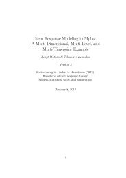
In this example, the confirmatory LCA with two categorical latent 

variables shown in the picture above is estimated. The two categorical 

latent variables are correlated and have their own sets of latent class 

indicators. 

177

CHAPTER 7 

The CLASSES option is used to assign names to the categorical latent 

variables in the model and to specify the number of latent classes in the 

model for each categorical latent variable. In the example above, there 

are two categorical latent variables cu and cy. The categorical latent 

variable cu has two latent classes and the categorical latent variable cy 

has three latent classes. PARAMETERIZATION=LOGLINEAR is used 

to specify associations among categorical latent variables. In the 

LOGLINEAR parameterization, the WITH option of the MODEL 

command is used to specify the relationships between the categorical 

latent variables. When a model has more than one categorical latent 

variable, MODEL followed by a label is used to describe the analysis 

model for each categorical latent variable. Labels are defined by using 

the names of the categorical latent variables. The categorical latent 

variable cu has four binary indicators u1 through u4. Their thresholds 

are specified to vary only across the classes of the categorical latent 

variable cu. The categorical latent variable cy has four continuous 

indicators y1 through y4. Their means are specified to vary only across 

the classes of the categorical latent variable cy. The default estimator 



used to select a different estimator. An explanation of the other 


Following is an alternative specification of the associations among cu 

and cy: 

cu#1 WITH cy#1 cy#2; 

where cu#1 refers to the first class of cu, cy#1 refers to the first class of 

cy, and cy#2 refers to the second class of cy. The classes of a 

categorical latent variable are referred to by adding to the name of the 

categorical latent variable the number sign (#) followed by the number 

of the class. This alternative specification allows individual parameters 

to be referred to in the MODEL command for the purpose of giving 

starting values or placing restrictions. 

178


EXAMPLE 7.15: LOGLINEAR MODEL FOR A THREE-WAY 

TABLE WITH CONDITIONAL INDEPENDENCE BETWEEN 

THE FIRST TWO VARIABLES 

TITLE: this is an example of a loglinear model 

for a three-way table with conditional 

independence between the first two 

variables 


VARIABLE: NAMES ARE u1 u2 u3 w; 

FREQWEIGHT = w; 


CLASSES = c1 (2) c2 (2) c3 (2); 


STARTS = 0; 

PARAMETERIZATION = LOGLINEAR; 

MODEL: 

%OVERALL% 

c1 WITH c3; 

c2 WITH c3; 

MODEL c1: 

%c1#1% 

[u1$1@15]; 

%c1#2% 

[u1$1@-15]; 

MODEL c2: 

%c2#1% 

[u2$1@15]; 

%c2#2% 

[u2$1@-15]; 

MODEL c3: 

%c3#1% 

[u3$1@15]; 

%c3#2% 

[u3$1@-15]; 


In this example, a loglinear model for a three-way frequency table with 

conditional independence between the first two variables is estimated. 

The loglinear model is estimated using categorical latent variables that 

are perfectly measured by observed categorical variables. It is also 

possible to estimate loglinear models for categorical latent variables that 

are measured with error by observed categorical variables. The 

conditional independence is specified by the two-way interaction 

179

CHAPTER 7 

between the first two variables being zero for each of the two levels of 

the third variable. 

PARAMETERIZATION=LOGLINEAR is used to estimate loglinear 

models with two- and three-way interactions. In the LOGLINEAR 

parameterization, the WITH option of the MODEL command is used to 

specify the associations among the categorical latent variables. When a 

model has more than one categorical latent variable, MODEL followed 

by a label is used to describe the analysis model for each categorical 

latent variable. Labels are defined by using the names of the categorical 

latent variables. In the example above, the categorical latent variables 

are perfectly measured by the latent class indicators. This is specified by 

fixing their thresholds to the logit value of plus or minus 15, 

corresponding to probabilities of zero and one. The default estimator for 

this type of analysis is maximum likelihood with robust standard errors. 

The ESTIMATOR option of the ANALYSIS command can be used to 

select a different estimator. An explanation of the other commands can 

be found in Examples 7.1 and 7.14. 

EXAMPLE 7.16: LCA WITH PARTIAL CONDITIONAL 

INDEPENDENCE 

TITLE: this is an example of LCA with partial 

conditional independence 




CLASSES = c(2); 


ALGORITHM = INTEGRATION; 

MODEL: 

%OVERALL% 

f by u2-u3@0; 

f@1; [f@0]; 

%c#1% 

[u1$1-u4$1*-1]; 

f by u2@1 u3; 


180


u1 

u2 

c 

u3 

f 

u4 

In this example, the LCA with partial conditional independence shown 

in the picture above is estimated. A similar model is described in Qu, 

Tan, and Kutner (1996). 

By specifying ALGORITHM=INTEGRATION, a maximum likelihood 

estimator with robust standard errors using a numerical integration 

algorithm will be used. Note that numerical integration becomes 

increasingly more computationally demanding as the number of factors 

and the sample size increase. In this example, one dimension of 

integration is used with 15 integration points. The ESTIMATOR option 

can be used to select a different estimator. In the example above, the 

lack of conditional independence between the latent class indicators u2 

and u3 in class 1 is captured by u2 and u3 being influenced by the 

continuous latent variable f in class 1. The conditional independence 

assumption for u2 and u3 is not violated for class 2. This is specified by 

fixing the factor loadings to zero in the overall model. The amount of 

deviation from conditional independence between u2 and u3 in class 1 is 

captured by the u3 factor loading for the continuous latent variable f. An 

explanation of the other commands can be found in Example 7.1. 

181

CHAPTER 7 

EXAMPLE 7.17: MIXTURE CFA MODELING 

TITLE: this is an example of mixture CFA modeling 



CLASSES = c(2); 



f BY y1-y5; 

%c#1% 

[f*1]; 


y1 y2 y3 y4 

y5 

c 

f 

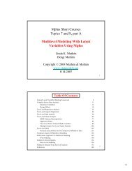
In this example, the mixture CFA model shown in the picture above is 

estimated (Muthén, 2008). The mean of the factor f varies across the 

classes of the categorical latent variable c. The residual arrow pointing 

to f indicates that the factor varies within class. This implies that the 

distribution of f is allowed to be non-normal. It is possible to allow 

other parameters of the CFA model to vary across classes. 

The BY statement specifies that f is measured by y1, y2, y3, y4, and y5. 

The factor mean varies across the classes. All other model parameters 

are held equal across classes as the default. The default estimator for 

this type of analysis is maximum likelihood with robust standard errors. 

The ESTIMATOR option of the ANALYSIS command can be used to 

select a different estimator. An explanation of the other commands can 

be found in Example 7.1. 

182


EXAMPLE 7.18: LCA WITH A SECOND-ORDER FACTOR 

(TWIN ANALYSIS) 

TITLE: this is an example of a LCA with a secondorder 

factor (twin analysis) 


VARIABLE: NAMES ARE u11-u13 u21-u23; 

CLASSES = c1(2) c2(2); 




MODEL: 

%OVERALL% 

f BY; 

f@1; 

c1 c2 ON f*1 (1); 

MODEL c1: 

%c1#1% 

[u11$1-u13$1*-1]; 

%c1#2% 

[u11$1-u13$1*1]; 

MODEL c2: 

%c2#1% 

[u21$1-u23$1*-1]; 

%c2#2% 

[u21$1-u23$1*1]; 


183

CHAPTER 7 

u11 u12 u13 

u21 u22 u23 

c1 

c2 

f 

In this example, the second-order factor model shown in the picture 

above is estimated. The first-order factors are categorical latent 

variables and the second-order factor is a continuous latent variable. 

This is a model that can be used for studies of twin associations where 

the categorical latent variable c1 refers to twin 1 and the categorical 

latent variable c2 refers to twin 2. 







can be used to select a different estimator. When a model has more than 

one categorical latent variable, MODEL followed by a label is used to 

describe the analysis model for each categorical latent variable. Labels 

are defined by using the names of the categorical latent variables. 

In the overall model, the BY statement names the second order factor f. 

The ON statement specifies that f influences both categorical latent 

variables in the same amount by imposing an equality constraint on the 

two multinomial logistic regression coefficients. The slope in the 

multinomial regression of c on f reflects the strength of association 

184


between the two categorical latent variables. An explanation of the 

other commands can be found in Examples 7.1 and 7.14. 

EXAMPLE 7.19: SEM WITH A CATEGORICAL LATENT 

VARIABLE REGRESSED ON A CONTINUOUS LATENT 

VARIABLE 

TITLE: this is an example of a SEM with a 

categorical latent variable regressed on a 

continuous latent variable 







MODEL: 

%OVERALL% 

f BY u1-u4; 

c ON f; 

%c#1% 

[u5$1-u8$1]; 

%c#2% 

[u5$1-u8$1]; 


u1 

u5 

u2 

u3 

f 

c 

u6 

u7 

u4 

u8 

185

CHAPTER 7 

In this example, the model with both a continuous and categorical latent 

variable shown in the picture above is estimated. The categorical latent 

variable c is regressed on the continuous latent variable f in a 

multinomial logistic regression. 







can be used to select a different estimator. In the overall model, the BY 

statement specifies that f is measured by the categorical factor indicators 

u1 through u4. The categorical latent variable c has four binary latent 

class indicators u5 through u8. The ON statement specifies the 

multinomial logistic regression of the categorical latent variable c on the 

continuous latent variable f. An explanation of the other commands can 

be found in Example 7.1. 

EXAMPLE 7.20: STRUCTURAL EQUATION MIXTURE 

MODELING 

TITLE: this is an example of structural equation 

mixture modeling 





MODEL: 

%OVERALL% 

f1 BY y1-y3; 

f2 BY y4-y6; 

f2 ON f1; 

%c#1% 

[f1*1 f2]; 

f2 ON f1; 


186


y1 

y4 

y2 

f1 

f2 

y5 

y3 

y6 

c 

In this example, the structural equation mixture model shown in the 

picture above is estimated. A continuous latent variable f2 is regressed 

on a second continuous latent variable f1. The solid arrows from the 

categorical latent variable c to f1 and f2 indicate that the mean of f1 and 

the intercept of f2 vary across classes. The broken arrow from c to the 

arrow from f1 to f2 indicates that the slope in the linear regression of f2 

on f1 varies across classes. For related models, see Jedidi, Jagpal, and 

DeSarbo (1997). 

In the overall model, the first BY statement specifies that f1 is measured 

by y1 through y3. The second BY statement specifies that f2 is 

measured by y4 through y6. The ON statement describes the linear 

regression of f2 on f1. In the model for class 1, the mean of f1, the 

intercept of f2, and the slope in the regression of f2 on f1 are specified to 

be free across classes. All other parameters are held equal across classes 

as the default. The default estimator for this type of analysis is 




Example 7.1. 

187

CHAPTER 7 

EXAMPLE 7.21: MIXTURE MODELING WITH KNOWN 

CLASSES (MULTIPLE GROUP ANALYSIS) 

TITLE: this is an example of mixture modeling 

with known classes (multiple group 

analysis) 


VARIABLE: NAMES = g y1-y4; 

CLASSES = cg (2) c (2); 

KNOWNCLASS = cg (g = 0 g = 1); 


MODEL: 

%OVERALL% 

c ON cg; 

MODEL c: 

%c#1% 

[y1-y4]; 

%c#2% 

[y1-y4]; 

MODEL cg: 

%cg#1% 

y1-y4; 

%cg#2% 

y1-y4; 


y1 y2 y3 y4 

cg 

c 

In this example, the multiple group mixture model shown in the picture 

above is estimated. The groups are represented by the classes of the 

categorical latent variable cg, which has known class (group) 

membership. 

188


The KNOWNCLASS option is used for multiple group analysis with 

TYPE=MIXTURE. It is used to identify the categorical latent variable 

for which latent class membership is known and is equal to observed 

groups in the sample. The KNOWNCLASS option identifies cg as the 

categorical latent variable for which latent class membership is known. 

The information in parentheses following the categorical latent variable 

name defines the known classes using an observed variable. In this 

example, the observed variable g is used to define the known classes. 

The first class consists of individuals with the value 0 on the variable g. 

The second class consists of individuals with the value 1 on the variable 

g. The means of y1, y2, y3, and y4 vary across the classes of c, while 

the variances of y1, y2, y3, and y4 vary across the classes of cg. An 


EXAMPLE 7.22: MIXTURE MODELING WITH CONTINUOUS 

VARIABLES THAT CORRELATE WITHIN CLASS 

(MULTIVARIATE NORMAL MIXTURE MODEL) 

TITLE: this is an example of mixture modeling 

with continuous variables that correlate 

within class (multivariate normal mixture 

model) 





MODEL: 

%OVERALL% 

y1 WITH y2-y4; 

y2 WITH y3 y4; 

y3 WITH y4; 

%c#2% 

[y1–y4*-1]; 

%c#3% 

[y1–y4*1]; 


189

CHAPTER 7 

y1 

y2 

c 

y3 

y4 

In this example, the mixture model shown in the picture above is 

estimated. Because c is a categorical latent variable, the interpretation of 

the picture is not the same as for models with continuous latent 

variables. The arrows from c to the observed variables y1, y2, y3, and 

y4 indicate that the means of the observed variables vary across the 

classes of c. The arrows correspond to the regressions of the observed 

variables on a set of dummy variables representing the categories of c. 

The observed variables correlate within class. This is a conventional 

multivariate mixture model (Everitt & Hand, 1981; McLachlan & Peel, 

2000). 

In the overall model, by specifying the three WITH statements the 

default of zero covariances within class is relaxed and the covariances 

among y1, y2, y3, and y4 are estimated. These covariances are held 

equal across classes as the default. The variances of y1, y2, y3, and y4 

are estimated and held equal as the default. These defaults can be 

overridden. The means of the categorical latent variable c are estimated 

as the default. 

When WITH statements are included in a mixture model, starting values 

may be useful. In the class-specific model for class 2, starting values of 

-1 are given for the means of y1, y2, y3, and y4. In the class-specific 

model for class 3, starting values of 1 are given for the means of y1, y2, 

190


y3, and y4. The default estimator for this type of analysis is maximum 

likelihood with robust standard errors. The ESTIMATOR option of the 

ANALYSIS command can be used to select a different estimator. An 


EXAMPLE 7.23: MIXTURE RANDOMIZED TRIALS 

MODELING USING CACE ESTIMATION WITH TRAINING 

DATA 

TITLE: this is an example of mixture randomized 

trials modeling using CACE estimation with 

training data 


VARIABLE: NAMES ARE y x1 x2 c1 c2; 


TRAINING = c1 c2; 


MODEL: 

%OVERALL% 

y ON x1 x2; 

c ON x1; 

%c#1% 

[y]; 

y; 

y ON x2@0; 

%c#2% 

[y*.5]; 

y; 


191

CHAPTER 7 

y 

c 

x1 

x2 

In this example, the mixture model for randomized trials using CACE 

(Complier-Average Causal Effect) estimation with training data shown 

in the picture above is estimated (Little & Yau, 1998). The continuous 

dependent variable y is regressed on the covariate x1 and the treatment 

dummy variable x2. The categorical latent variable c is compliance 

status, with class 1 referring to non-compliers and class 2 referring to 

compliers. Compliance status is observed in the treatment group and 

unobserved in the control group. Because c is a categorical latent 

variable, the interpretation of the picture is not the same as for models 

with continuous latent variables. The arrow from c to the y variable 

indicates that the intercept of y varies across the classes of c. The arrow 

from c to the arrow from x2 to y indicates that the slope in the regression 

of y on x2 varies across the classes of c. The arrow from x1 to c 

represents the multinomial logistic regression of c on x1. 

The TRAINING option is used to identify the variables that contain 

information about latent class membership. Because there are two 

classes, there are two training variables c1 and c2. Individuals in the 

treatment group are assigned values of 1 for c1 and 0 for c2 if they are 

non-compliers and 0 for c1 and 1 for c2 if they are compliers. 

Individuals in the control group are assigned values of 1 for both c1 and 

192


c2 to indicate that they are allowed to be a member of either class and 

that their class membership is estimated. 

In the overall model, the first ON statement describes the linear 

regression of y on the covariate x1 and the treatment dummy variable x2. 

The intercept and residual variance of y are estimated as the default. 

The second ON statement describes the multinomial logistic regression 

of the categorical latent variable c on the covariate x1 when comparing 

class 1 to class 2. The intercept in the regression of c on x1 is estimated 

as the default. 

In the model for class 1, a starting value of zero is given for the intercept 

of y as the default. The residual variance of y is specified to relax the 

default across class equality constraint. The ON statement describes the 

linear regression of y on x2 where the slope is fixed at zero. This is 

done because non-compliers do not receive treatment. In the model for 

class 2, a starting value of .5 is given for the intercept of y. The residual 

variance of y is specified to relax the default across class equality 

constraint. The regression of y ON x2, which represents the CACE 

treatment effect, is not fixed at zero for class 2. The default estimator 



used to select a different estimator. An explanation of the other 


EXAMPLE 7.24: MIXTURE RANDOMIZED TRIALS 

MODELING USING CACE ESTIMATION WITH MISSING 

DATA ON THE LATENT CLASS INDICATOR 

TITLE: this is an example of mixture randomized 

trials modeling using CACE estimation with 

missing data on the latent class indicator 


VARIABLE: NAMES ARE u y x1 x2; 


CATEGORICAL = u; 

MISSING = u (999); 


193

CHAPTER 7 

MODEL: 

%OVERALL% 

y ON x1 x2; 

c ON x1; 

%c#1% 

[u$1@15]; 

[y]; 

y; 

y ON x2@0; 

OUTPUT: 

%c#2% 

[u$1@-15]; 

[y*.5]; 

y; 

TECH1 TECH8; 

u 

y 

c 

x1 

x2 

The difference between this example and Example 7.23 is that a binary 

latent class indicator u has been added to the model. This binary 

variable represents observed compliance status. Treatment compliers 

have a value of 1 on this variable; treatment non-compliers have a value 

of 0 on this variable; and individuals in the control group have a missing 

value on this variable. The latent class indicator u is used instead of 

training data. 

194


In the model for class 1, the threshold of the latent class indicator 

variable u is set to a logit value of 15. In the model for class 2, the 

threshold of the latent class indicator variable u is set to a logit value of 

–15. These logit values reflect that c is perfectly measured by u. 

Individuals in the non-complier class (class 1) have probability zero of 

observed compliance and individuals in the complier class (class 2) have 

probability one of observed compliance. The default estimator for this 

type of analysis is maximum likelihood with robust standard errors. The 




EXAMPLE 7.25: ZERO-INFLATED POISSON REGRESSION 

CARRIED OUT AS A TWO-CLASS MODEL 

TITLE: this is an example of a zero-inflated 

Poisson regression carried out as a twoclass 

model 


VARIABLE: NAMES ARE u1 x1 x3; 

COUNT IS u1; 



MODEL: 

%OVERALL% 

u1 ON x1 x3; 

c ON x1 x3; 

%c#1% 

[u1@-15]; 

u1 ON x1@0 x3@0; 


x1 

u1 

x3 

c 

195

CHAPTER 7 

In this example, the zero-inflated Poisson regression model shown in the 

picture above is estimated. This is an alternative to the way zeroinflated 

Poisson regression was carried out in Example 3.8. In the 

example above, a categorical latent variable c with two classes is used to 

represent individuals who are able to assume values of zero and above 

and individuals who are unable to assume any value except zero. The 

categorical latent variable c corresponds to the binary latent inflation 

variable u1#1 in Example 3.8. This approach has the advantage of 

allowing the estimation of the probability of being in each class and the 

posterior probabilities of being in each class for each individual. 

The COUNT option is used to specify which dependent variables are 

treated as count variables in the model and its estimation and whether a 

Poisson or zero-inflated Poisson model will be estimated. In the 

example above, u1 is a specified as count variable without inflation 

because the inflation is captured by the categorical latent variable c. 

In the overall model, the first ON statement describes the Poisson 

regression of the count variable u1 on the covariates x1 and x3. The 

second ON statement describes the multinomial logistic regression of the 

categorical latent variable c on the covariates x1 and x3 when comparing 

class 1 to class 2. In this example, class 1 contains individuals who are 

unable to assume any value except zero on u1. Class 2 contains 

individuals whose values on u1 are distributed as a Poisson variable 

without inflation. Mixing the two classes results in u1 having a zeroinflated 

Poisson distribution. In the class-specific model for class 1, the 

intercept of u1 is fixed at -15 to represent a low log rate at which the 

probability of a count greater than zero is zero. Therefore, all 

individuals in class 1 have a value of 0 on u1. Because u1 has no 

variability, the slopes in the Poisson regression of u1 on the covariates 

x1 and x3 in class 1 are fixed at zero. The default estimator for this type 

of analysis is maximum likelihood with robust standard errors. The 



found in Example 7.1. 

196


EXAMPLE 7.26: CFA WITH A NON-PARAMETRIC 

REPRESENTATION OF A NON-NORMAL FACTOR 

DISTRIBUTION 

TITLE: this is an example of CFA with a nonparametric 

representation of a non-normal 

factor distribution 


VARIABLE: NAMES ARE y1-y5 c; 

USEV = y1-y5; 




f BY y1-y5; 

f@0; 


In this example, a CFA model with a non-parametric representation of a 

non-normal factor distribution is estimated. One difference between this 

example and Example 7.17 is that the factor variance is fixed at zero in 

each class. This is done to capture a non-parametric representation of 

the factor distribution (Aitkin, 1999) where the latent classes are used to 

represent non-normality not unobserved heterogeneity with substantively 

meaningful latent classes. This is also referred to as semiparametric 

modeling. The factor distribution is represented by a histogram with as 

many bars as there are classes. The bars represent scale steps on the 

continuous latent variable. The spacing of the scale steps is obtained by 

the factor means in the different classes with a factor mean for one class 

fixed at zero for identification, and the percentage of individuals at the 

different scale steps is obtained by the latent class percentages. This 

means that continuous factor scores are obtained for the individuals 

while not assuming normality for the factor but estimating its 

distribution. Factor variances can also be estimated to obtain a more 

general mixture although this reverts to the parametric assumption of 

normality, in this case, within each class. When the latent classes are 

used to represent non-normality, the mixed parameter values are of 

greater interest than the parameters for each mixture component 

(Muthén, 2002, p. 102; Muthén, 2004). An explanation of the other 


197

CHAPTER 7 

EXAMPLE 7.27: FACTOR (IRT) MIXTURE ANALYSIS WITH 

BINARY LATENT CLASS AND FACTOR INDICATORS 

TITLE: this is an example of a factor (IRT) 

mixture analysis with binary latent class 

and factor indicators 

DATA: FILE = ex7.27.dat; 

VARIABLE: NAMES = u1-u8; 





STARTS = 100 20; 


f BY u1-u8; 

[f@0]; 

%c#1% 

f BY u1@1 u2-u8; 

f; 

[u1$1-u8$1]; 

%c#2% 

f BY u1@1 u2-u8; 

f; 

[u1$1-u8$1]; 


u1 u2 u3 u4 u5 u6 u7 u8 

c 

f 

198


In this example, the factor (IRT) mixture model shown in the picture 

above is estimated (Muthén, 2008). The model is a generalization of the 

latent class model where the latent class model assumption of 

conditional independence between the latent class indicators within class 

is relaxed using a factor that influences the items within each class 

(Muthén, 2006; Muthén & Asparouhov, 2006; Muthén, Asparouhov, & 

Rebollo, 2006). The factor represents individual variation in response 

probabilities within class. Alternatively, this model may be seen as an 

Item Response Theory (IRT) mixture model. The broken arrows from 

the categorical latent variable c to the arrows from the factor f to the 

latent class indicators u1 to u8 indicate that the factor loadings vary 

across classes. 







can be used to select a different estimator. The STARTS option is used 

to specify the number of initial stage random sets of starting values to 

generate and the number of final stage optimizations to use. The default 

is 20 random sets of starting values for the initial stage and 4 

optimizations for the final stage. In the example above, the STARTS 

option specifies that 100 random sets of starting values for the initial 

stage and 20 final stage optimizations will be used. 

In the overall model, the BY statement specifies that the factor f is 

measured by u1, u2, u3, u4, u5, u6, u7, and u8. The mean of the factor is 

fixed at zero which implies that the mean is zero in both classes. The 

factor variance is held equal across classes as the default. The 

statements in the class-specific parts of the model relax the equality 

constraints across classes for the factor loadings, factor variance, and the 

thresholds of the indicators. An explanation of the other commands can 

be found in Examples 7.1 and 7.3. 

199

CHAPTER 7 

EXAMPLE 7.28: TWO-GROUP TWIN MODEL FOR 

CATEGORICAL OUTCOMES USING MAXIMUM 

LIKELIHOOD AND PARAMETER CONSTRAINTS 

TITLE: this is an example of a two-group twin 

model for categorical outcomes using 

maximum likelihood and parameter 

constraints 


VARIABLE: NAMES = u1 u2 dz; 

CATEGORICAL = u1 u2; 

CLASSES = cdz (2); 

KNOWNCLASS = cdz (dz = 0 dz = 1); 



LINK = PROBIT; 

MODEL: 

%OVERALL% 

[u1$1-u2$1] (1); 

f1 BY u1; 

f2 BY u2; 

[f1-f2@0]; 

f1-f2 (varf); 

%cdz#1% 

f1 WITH f2(covmz); 

%cdz#2% 

f1 WITH f2(covdz); 


NEW(a c h); 

varf = a**2 + c**2 + .001; 

covmz = a**2 + c**2; 

covdz = 0.5*a**2 + c**2; 

h = a**2/(a**2 + c**2 + 1); 

200


u1 

u2 

f1 

f2 

In this example, the model shown in the picture above is estimated. The 

variables u1 and u2 represent a univariate outcome for each member of a 

twin pair. Monozygotic and dizygotic twins are considered in a twogroup 

twin model for categorical outcomes using maximum likelihood 

estimation. Parameter constraints are used to represent the ACE model 

restrictions. The ACE variance and covariance restrictions are placed on 

normally-distributed latent response variables, which are also called 

liabilities, underlying the categorical outcomes. This model is referred 

to as the threshold model for liabilities (Neale & Cardon, 1992). The 

monozygotic and dizygotic twin groups are represented by latent classes 

with known class membership. 



in the model and its estimation. In the example above, the variables u1 

and u2 are binary or ordered categorical variables. The program 

determines the number of categories for each indicator. The 

KNOWNCLASS option identifies cdz as the categorical latent variable 

for which latent class membership is known. The information in 

parentheses following the categorical latent variable name defines the 

known classes using an observed variable. In this example, the observed 

variable dz is used to define the known classes. The first class consists 

of the monozygotic twins who have the value 0 on the variable dz. The 

second class consists of the dizygotic twins who have the value 1 on the 

variable dz. 



201

CHAPTER 7 



and the sample size increase. In this example, two dimensions of 

integration are used with 225 integration points. The ESTIMATOR 

option can be used to select a different estimator. The LINK option is 

used with maximum likelihood estimation to select a logit or a probit 

link for models with categorical outcomes. The default is a logit link. In 

this example, the probit link is used because the threshold model for 

liabilities uses normally-distributed latent response variables. 

In the overall model, the (1) following the first bracket statement 

specifies that the thresholds of u1 and u2 are held equal across twins. 

The two BY statements define a factor behind each outcome. This is 

done because covariances of categorical outcomes are not part of the 

model when maximum likelihood estimation is used. The covariances of 

the factors become the covariances of the categorical outcomes or more 

precisely the covariances of the latent response variables underlying the 

categorical outcomes. The means of the factors are fixed at zero and 

their variances are held equal across twins. The variance of each 

underlying response variable is obtained as the sum of the factor 

variance plus one where one is the residual variance in the probit 

regression of the categorical outcome on the factor. 

In the MODEL command, labels are defined for three parameters. The 

label varf is assigned to the variances of f1 and f2. Because they are 

given the same label, these parameters are held equal. The label covmz 

is assigned to the covariance between f1 and f2 for the monozygotic 

twins and the label covdz is assigned to the covariance between f1 and f2 

for the dizygotic twins. In the MODEL CONSTRAINT command, the 

NEW option is used to assign labels to three parameters that are not in 

the analysis model: a, c, and h. The two parameters a and c are used to 

decompose the covariances of u1 and u2 into genetic and environmental 

components. The value .001 is added to the variance of the factors to 

avoid a singular factor covariance matrix which comes about because the 

factor variances and covariances are the same. The parameter h does not 

impose restrictions on the model parameters but is used to compute the 

heritability estimate and its standard error. This heritability estimate 

uses the residual variances for the latent response variables which are 

fixed at one. An explanation of the other commands can be found in 

Example 7.1. 

202


EXAMPLE 7.29: TWO-GROUP IRT TWIN MODEL FOR 

FACTORS WITH CATEGORICAL FACTOR INDICATORS 

USING PARAMETER CONSTRAINTS 

TITLE: this is an example of a two-group IRT twin 

model for factors with categorical factor 

indicators using parameter constraints 


VARIABLE: NAMES = u11-u14 u21-u24 dz; 


CLASSES = cdz (2); 

KNOWNCLASS = cdz (dz = 0 dz = 1); 



MODEL: 

%OVERALL% 

f1 BY u11 

u12-u14 (lam2-lam4); 

f2 BY u21 

u22-u24 (lam2-lam4); 

[f1-f2@0]; 

f1-f2 (var); 

[u11$1-u14$1] (t1-t4); 

[u21$1-u24$1] (t1-t4); 

%cdz#1% 

f1 WITH f2(covmz); 

%cdz#2% 

f1 WITH f2(covdz); 


NEW(a c e h); 

var = a**2 + c**2 + e**2; 

covmz = a**2 + c**2; 

covdz = 0.5*a**2 + c**2; 

h = a**2/(a**2 + c**2 + e**2); 

203

CHAPTER 7 

u11 u12 u13 u14 

u21 u22 u23 u24 

f1 

f2 

In this example, the model shown in the picture above is estimated. The 

factors f1 and f2 represent a univariate variable for each member of the 

twin pair. Monozygotic and dizygotic twins are considered in a twogroup 

twin model for factors with categorical factor indicators using 

parameter constraints and maximum likelihood estimation. Parameter 

constraints are used to represent the ACE model restrictions. The ACE 

variance and covariance restrictions are placed on two factors instead of 

two observed variables as in Example 7.28. The relationships between 

the categorical factor indicators and the factors are logistic regressions. 

Therefore, the factor model for each twin is a two-parameter logistic 

Item Response Theory model (Muthén, Asparouhov, & Rebollo, 2006). 

The monozygotic and dizygotic twin groups are represented by latent 

classes with known class membership. 





and the sample size increase. In this example, two dimensions of 

integration are used with 225 integration points. The ESTIMATOR 

option can be used to select a different estimator. 

In the overall model, the two BY statements specify that f1 is measured 

by u11, u12, u13, and u14 and that f2 is measured by u21, u22, u23, and 

u24. The means of the factors are fixed at zero. In the class-specific 

models, the threshold of the dz variable is fixed at 15 in class one and - 

15 in class 2. 

204


In the MODEL command, labels are defined for nine parameters. The 

list function can be used when assigning labels. The label lam2 is 

assigned to the factor loadings for u12 and u22; the label lam3 is 

assigned to the factor loadings for u13 and u23; and the label lam4 is 

assigned to the factor loadings for u14 and u24. Factor loadings with the 

same label are held equal. The label t1 is assigned to the thresholds of 

u11 and u21; the label t2 is assigned to the thresholds of u12 and u22; 

the label t3 is assigned to the thresholds of u13 and u23; and the label t4 

is assigned to the thresholds of u14 and u24. Parameters with the same 

label are held equal. The label covmz is assigned to the covariance 

between f1 and f2 for the monozygotic twins and the label covdz is 

assigned to the covariance between f1 and f2 for the dizygotic twins. 

In the MODEL CONSTRAINT command, the NEW option is used to 

assign labels to four parameters that are not in the analysis model: a, c, 

e, and h. The three parameters a, c, and e are used to decompose the 

variances and covariances of f1 and f2 into genetic and environmental 

components. The parameter h does not impose restrictions on the model 

parameters but is used to compute the heritability estimate and its 

standard error. An explanation of the other commands can be found in 

Examples 7.1 and 7.28. 

EXAMPLE 7.30: CONTINUOUS-TIME SURVIVAL ANALYSIS 

USING A COX REGRESSION MODEL TO ESTIMATE A 

TREATMENT EFFECT 

TITLE: this is an example of continuous-time 

survival analysis using a Cox regression 

model to estimate a treatment effect 


VARIABLE: NAMES are t u x tcent class; 

USEVARIABLES = t-tcent; 

SURVIVAL = t; 

TIMECENSORED = tcent; 

CATEGORICAL = u; 



205

CHAPTER 7 

MODEL: 

OUTPUT: 

PLOT: 

%OVERALL% 

t ON x; 

%c#1% 

[u$1@15]; 

[t@0]; 

%c#2% 

[u$1@-15]; 

[t]; 

TECH1 LOGRANK; 

TYPE = PLOT2; 

u 

t 

c 

x 

In this example, the continuous-time survival analysis model shown in 

the picture above is estimated. The model is similar to Larsen (2004). A 

treatment and a control group are analyzed as two known latent classes. 

The baseline hazards are held equal across the classes and the treatment 

effect is expressed as the intercept of the survival variable in the 

treatment group. For applications of this model, see Muthén et al. 

(2009). 

The CATEGORICAL option is used to specify that the variable u is a 

binary variable. This variable is a treatment dummy variable where zero 

represents the control group and one represents the treatment group. In 

this example, the categorical latent variable c has two classes. In the 

MODEL command, in the model for class 1, the threshold for u is fixed 

at 15 so that the probability that u equals one is zero. By this 

206


specification, class 1 is the control group. In the model for class 2, the 

threshold for u is fixed at -15 so that the probability that u equals one is 

one. By this specification, class 2 is the treatment group. In the overall 

model, the ON statement describes the Cox regression for the survival 

variable t on the covariate x. In class 1, the intercept in the Cox 

regression is fixed at zero. In class 2, it is free. This intercept represents 

the treatment effect. The LOGRANK option of the OUTPUT command 

provides a logrank test of the equality of the treatment and control 

survival curves (Mantel, 1966). By specifying PLOT2 in the PLOT 

command, the following plots are obtained: 

• Kaplan-Meier curve 

• Sample log cumulative hazard curve 

• Estimated baseline hazard curve 

• Estimated baseline survival curve 

• Estimated log cumulative baseline curve 

• Kaplan-Meier curve with estimated baseline survival curve 

• Sample log cumulative hazard curve with estimated log 

cumulative baseline curve 

An explanation of the other commands can be found in Example 7.1. 

207

CHAPTER 7 

208

EXAMPLES: MIXTURE MODELING WITH CROSS ... - Mplus

You also want an ePaper? Increase the reach of your titles

Delete template?

Save as template?