AE/ME 201-- Procedure -- Lab: Tank Draining Instrumentation and ...

AE/ME 201 – Spring 2005
Tank Draining Instrumentation and Calculation of Exit Losses
R. S. LaFleur and J. A. Taylor ∗
Mech. & Aero. Eng. Dept.
Clarkson University Box 5725
Potsdam, NY 13699-5725
Purpose:
This experiment is intended to support the Differential
Equations course. The student will instrument
a tank and measure the loss coefficient, C, that relates
the height fluid in the tank to the the velocity
of the free surface as the tank drains. This relationship
is described by a first order differential equation
of the form:
dh
dt = C2 h (1)
and in addition to determining the loss coefficient,
C, the student will have to evaluate the uncertainty
in his or her estimate of C.
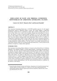
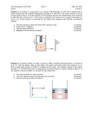
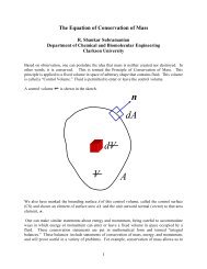
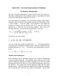
Figure 1: Side view of the immersion probe.
Background:
The background information for this experiment
will be separated into two subsections. The first
will focus on the instrumentation and the second
will attempt to describe how the differential equation
that we’re attempting to solve was obtained.
Instrumentation
Please read pages 203-208 (Wheatstone bridge – deflection
method), 235-243 (data acquisition), 438-
439 (strain gauge electrical circuits) in the text [1] .
Two metal rods separated by an insulator are used
to sense water height or level in a tank. This simple
sensor has no moving parts. When immersed in
water, the rods and water between the rods forms
an electrical resistor. The resistance, R, of the
probe is calculated from the resistivity of the water,
r, the distance apart the rods are spaced, L, and the
wetted conduction area, A which, in turn, depends
upon the depth of the probe, d and a field factor,
η. The field factor η is a function of the resistance
∗ taylorja@clarkson.edu, (315) 268-6683, and CAMP 266
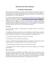
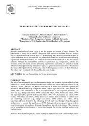
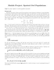
Figure 2: Top view of the immeersion probe.
of the water which varies with suspended impurities
and will require us to perform a calibration before
performing our experiment.
R probe = rL A = rL
ηd
(2)
We can see from equation 2 that the probe resistance
will increase as the depth of probe, or the
height of the water, decreases. The immersion probe
will form one leg of a wheatstone bridge circuit and
as the resistance of the probe changes, the bridge
output voltage will indicate the change in the height
of the water from its initial height.
The change in bridge output is small but sufficiently
large that the response can be acquired using a digital
data acquisition system. The DAQ system can
rapidly record the deflected bridge output. This
speed is required to resolve the transient level within
1

AE/ME 201 – Spring 2005
the tank.
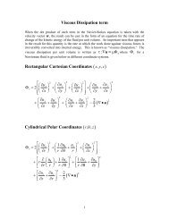
7. ρ - density
With 3 locations and 7 unknowns at each, there are
a total of 21 unknowns initially.
Using a definition of total pressure from the
Bernoulli equation (not used yet), one definition
links four of the quantities for each location. The
three state equations are:
P T1 = P s1 + ρ 1V1
2
2
+ ρ 1 gh 1 (3)
Fluid Mechanics
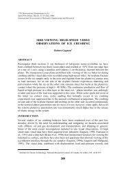
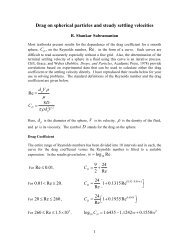
Figure 3: Schematic of tank.
Although, this experiment is intended to introduce
you to some different instrumentation techniques
and demonstrate experimental methods for obtaining
the constant coefficient in a simple first order
differential equation, a brief introduction to fluid
mechanics is included to help to understand what
you’re measuring and why.
Measurements of the liquid height versus time for
the tank draining will provide you with information
on the exit flow fixture (i.e. for your experiment,
this includes the section of pipe and the valve). For
example, the valve at the bottom of the tank provides
some resistance to flow and controls the rate
of draining and the rate of change of height versus
time. Also, the height in the tank sets the water
source pressure that drives the flow through the
valve. Therefore, the measurement of height versus
time provides an indication of both flow rate and
supply pressure.
There are three locations in question as shown in
Figure 3. At each location, seven quantities are used
to describe the state of the water or conditions:
1. P s - Static pressure
2. P T - Total pressure
3. V - flow velocity
4. h - fluid height
5. ṁ - mass flow
6. A - area
P T2 = P s2 + ρ 2V2
2
2
+ ρ 2 gh 2 (4)
P T3 = P s3 + ρ 3V3
2
+ ρ 3 gh 3 (5)
2
Conservation of mass applies between pairs of locations.
The two conservation of mass equations are:
and
ṁ 2 = ṁ 3 (6)
dh 1
ρ 1 A 1 = −ṁ 3 (7)
dt
Additional definitions are used to link some of the
quantities. The velocity at location 1 is the free
surface motion:
V 1 = dh 1
(8)
dt
Mass flow rates are defined from surface fluxes as:
and
ṁ 2 = ρ 2 A 2 V 2 (9)
ṁ 3 = ρ 3 A 3 V 3 (10)
The loss coefficient, K or K 23 , for the exit plumbing
(including the test section) is
K = K 23 = 2(P T 2
− P T3 )
ρ 2 V 2
2
This adds an unknown and an equation.
(11)
More equations are obtained by adopting some assumptions.
1. The total pressure loss between stations 1 and
2 is very small
2. density is constant and known - this is three
equations
3. The static pressure at station 1 is the local atmospheric
pressure
4. The static pressure at station 3 is the local atmospheric
pressure
2

5. All areas are given or measured - this is three
equations
6. Stations 2 and 3 are at a zero height reference
7. There is no mass flow at station 1
These add twelve equations. Adding all equations,
there are 20 equations total. Against 21 unknowns,
this leaves one degree of freedom. This will be the
initial height of station 1 when the exit valve is open.
With some algebra, dropping the subscript 1 from
h, some of these equations can be combined and manipulated
to solve for a first order differential equation
that governs the water height. This differential
equation is:
Instrumentation:
AE/ME 201 – Spring 2005
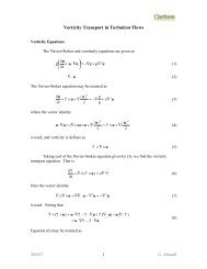
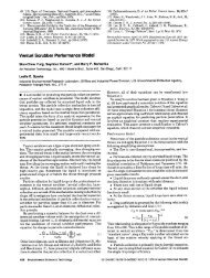
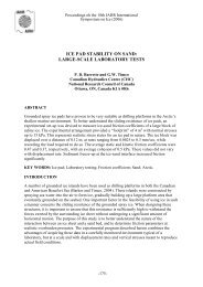
1. The HAMPTON instrumentation circuitry box
will be used to form a wheatstone bridge with
the probe as shown in Figure 4.
Voltage Supply: Sine Wave
Generator on the BNC-2120
Interface Box
V 1 = dh 1
= −C √ h (12)
dt
where C is defined as:
C 2 2g
=
K 23 ( A1
A 2
) 2 + ( A1
A 3
) 2 − 1 > 0 (13)
Notice that the fluid density does not appear anywhere
in equations 12 or 13.
From the traditional math-solution approach, the
loss coefficient, K, is specified along with all other
parameters and C is assumed constant over time
such that h(t) is solved. Unfortunately, we don’t
know enough about the resistance of the exit to
solve this problem directly. However, by using the
DAQ system to measure h(t), with a fine enough
time increment to accurately compute the rate of
change of h, C can be calculated. With fixed geometry
and water density, the loss coefficient, K, can
be also be determined.
C 2 = 1 ( dh )
(14)
h dt
where
K =
( A2
) 2 [ 2g
] (
A 1 C 2 + 1 A2
) 2
−
(15)
A 3
Experiment Apparatus:
Physical Hardware:
1. Fill a water tank to near the top with water.
Make sure the water level covers most of the
immersion probe as it hangs from the edge of
the tank. The dimensions of the tank should
be measured to enable volume calculations.
2. A few tablespoons of table salt should be added
to the tank. This will increase the conductivity
of the water.
Output Signal: Connect to
ACH5 on the BNC-2120
Interface Box
Figure 4: Circuit diagram – From: it Hampden
Model H-IT-2 Student Manual, (2002) Hampden
Engineering Corporation, pp. 50.
2. The bridge excitation will be provided by the
sine wave signal generator located on the lowest
row of BNC connectors on the NATIONAL
INSTRUMENTS interface module.
Procedures:
Lab partners will be positioned on opposite sides
of the work bench, and clear communication will
be necessary to coordinate tank draining and data
acquisition. You will begin by constructing the
Wheatstone bridge circuit. Then the you calibrate
the probe and perform the experiment.
Constructing the Circuits
1. Wire the power cable from sine wave generator
on the NATIONAL INSTRUMENTS interface
to the wheatstone bridge input. Place
3

AE/ME 201 – Spring 2005
the multi-meter in frequency mode and measure
the frequency provided.
2. The bridge excitation should be set to approximately:
±2VAC @ 5000Hz
3. Wire the bridge circuit including the immersion
probe.
4. Place the multimeter leads on the bridge output.
Set the multi-meter to AC function using
the voltage setting and switching the function
button (it looks like a little sine wave) on the
left side. The liquid crystal display should show
that AC is being measured.
5. Place the immersion probe in the water in the
tank and use the meter stick to measure the
liquid level.
6. Balance the bridge by adjusting the trim potentiometer,
P1, in the bridge ciruit. Zero may
not be obtained but the AC reading on the voltmeter
should be minimized.
7. Connect the output cable from ports J8 and
J12 to the BNC port labeled ACH5 on the NA-
TIONAL INSTRUMENTS interface.
Calibration
1. Insure that the drain will run into a bucket and
not onto the floor.
2. Launch the LabVIEW Vi, and press the run
arrow in the upper left corner of the screen.
You should see a sine wave displayed in one of
the plots and a voltage in the digital display in
the upper left hand portion of the screen.
3. Measure the initial water level.
4. Record the voltage shown in the display on
LABVIEW VI. The current voltage is displayed
in the ”liquid level” text box in the upper left
hand corner of the acquisition window.
5. Slowly drain a small amount of water into the
catch bucket. Measure the new water level.
6. Repeat steps 4 and 5 until the immersion probe
is nearly uncovered.
Tank Draining Test
1. Insure that the drain will run into a bucket and
not onto the floor.
2. Open the drain valve briefly and a small
amount to insure the trap is filled
3. Start the data acquisition routine by pressing
the run arrow in the upper left hand corner of
the screen. The output should appear in the
upper plot and a Fourier transformed version
of the output appears in the middle plot as a
spike at 5kHz. The lower plot will appear when
you begin storing the data.
4. To begin the data acquisition click the toggle
switch or button beneath the liquid level indicator
text box. Allow the system to acquire a
few seconds worth of data and then open the
drain valve fully to begin draining the tank.
5. Close the drain valve when the probe reading
reaches approximately 0.1V or the water
level drops below the bottom of the immersion
probe.
6. Stop the data acquisition by clicking the toggle
switch again, or by clicking the stop button,
and save the data onto disk. Your data file will
contain two columns: time and voltage.
7. Refill the tank to the starting level and repeat
the test procedure with the valve half open.
Software
A LabVIEW virtual instrument titled “Tank Draining”
is available within the “MAE Lab Software”
folder on the desktop for use with this experiment.
Tasks:
1. Plot the calibration data: the immersion probe
depth as a function of the voltage. Be sure to
include error bars on your data.
2. Perform a least squares fit of the calibration
curve to obtain a calibration formula and plot
a sample curve onto the plot of Task 1 to show
the quality of your data. NOTE: the calibration
curve is not linear, so you should use either an
exponential or a polynomial least squares fit.
3. Use the calibration curve formula to convert
voltage data to immersion probe depth. Plot
your calibrated data as a function of time.
4. Compute the derivative dh/dt to obtain the
draining velocity and construct a plot of the
velocity as a function of time.
4

AE/ME 201 – Spring 2005
5. Using the geometry of the tank and exit piping
and immersion probe depth versus time calculate
the K and its associated uncertainty, e K ,
for the exit. The Kline-McKlintock method [1]
of assessing the propagation of uncertainty to
a result should be used to compute e K .
References:
1. Taylor, J.A. (2004) “Uncertainty Analysis,”
http://www.clarkson.edu/class/maelab/
5