Data Compression Techniques in Wireless Sensor Networks
Data Compression Techniques in Wireless Sensor Networks
Data Compression Techniques in Wireless Sensor Networks

Create successful ePaper yourself
Turn your PDF publications into a flip-book with our unique Google optimized e-Paper software.
PERVASIVE COMPUTING 1<br />
<strong>Data</strong> <strong>Compression</strong> <strong>Techniques</strong> <strong>in</strong><br />
<strong>Wireless</strong> <strong>Sensor</strong> <strong>Networks</strong><br />
You-Chiun Wang<br />
Abstract—<strong>Wireless</strong> sensor networks (WSNs) open a new research field for pervasive comput<strong>in</strong>g and context-aware monitor<strong>in</strong>g of the<br />
physical environments. Many WSN applications aim at long-term environmental monitor<strong>in</strong>g. In these applications, energy consumption is a<br />
pr<strong>in</strong>cipal concern because sensor nodes have to regularly report their sens<strong>in</strong>g data to the remote s<strong>in</strong>k(s) for a very long time. S<strong>in</strong>ce data<br />
transmission is one primary factor of the energy consumption of sensor nodes, many research efforts focus on reduc<strong>in</strong>g the amount of data<br />
transmissions through data compression techniques. In this chapter, we discuss the data compression techniques <strong>in</strong> WSNs, which can be<br />
classified <strong>in</strong>to five categories: 1) The str<strong>in</strong>g-based compression techniques treat sens<strong>in</strong>g data as a sequence of characters and then adopt<br />
the text data compression schemes to compress them. 2) The image-based compression techniques hierarchically organize WSNs and<br />
then borrow the idea from the image compression solutions to handle sens<strong>in</strong>g data. 3) The distributed source cod<strong>in</strong>g techniques extend the<br />
Slepian-Wolf theorem to encode multiple correlated data streams <strong>in</strong>dependently at sensor nodes and then jo<strong>in</strong>tly decode them at the s<strong>in</strong>k. 4)<br />
The compressed sens<strong>in</strong>g techniques adopt a small number of nonadaptive and randomized l<strong>in</strong>ear projection samples to compress sens<strong>in</strong>g<br />
data. 5) The data aggregation techniques select a subset of sensor nodes <strong>in</strong> the network to be responsible for fus<strong>in</strong>g the sens<strong>in</strong>g data from<br />
other sensor nodes to reduce the amount of data transmissions. A comparison of these data compression techniques is also given <strong>in</strong> this<br />
chapter.<br />
Index Terms—compressed sens<strong>in</strong>g, data compression, data aggregation, distributed source cod<strong>in</strong>g, Slepian-Wolf theorem, wavelet<br />
transformation, wireless sensor networks.<br />
✦<br />
1 INTRODUCTION<br />
A wireless sensor network (WSN) is composed of one or<br />
several remote s<strong>in</strong>ks and a sheer number of sensor nodes.<br />
Each sensor node is a small, wireless device that can<br />
cont<strong>in</strong>ually collect its surround<strong>in</strong>g <strong>in</strong>formation and report<br />
the sens<strong>in</strong>g data to the s<strong>in</strong>k(s) through a multi-hop ad<br />
hoc rout<strong>in</strong>g scheme [1]. WSNs provide a new opportunity<br />
for pervasive comput<strong>in</strong>g and context-aware monitor<strong>in</strong>g of<br />
the physical environments. They are usually deployed <strong>in</strong><br />
regions of <strong>in</strong>terest to observe specific phenomena or track<br />
objects. Practical applications of WSNs <strong>in</strong>clude, for example,<br />
animal monitor<strong>in</strong>g, agriculture transform<strong>in</strong>g, health<br />
care, <strong>in</strong>door surveillance, and smart build<strong>in</strong>gs [2]–[6].<br />
Because sensor nodes are usually powered by batteries<br />
and many WSN applications aim at long-term monitor<strong>in</strong>g<br />
of the environments, how to conserve the energy of<br />
sensor nodes to extend their lifetimes is a critical issue.<br />
There are two common solutions to conserve the energy of<br />
sensor nodes. One solution is to take advantage of node<br />
redundancy by select<strong>in</strong>g a subset of sensor nodes to be<br />
active while putt<strong>in</strong>g others to sleep to conserve their energy<br />
[7]–[9]. The selected subset of active sensor nodes have<br />
to cover the whole monitor<strong>in</strong>g region and ma<strong>in</strong>ta<strong>in</strong> the<br />
network connectivity. In other words, these active sensor<br />
nodes have to make sure that the network still functions<br />
as well as the case when all sensor nodes are active. By<br />
select<strong>in</strong>g different subsets of sensor nodes to be active by<br />
turns, we can prevent some sensor nodes from consum<strong>in</strong>g<br />
too much energy and thus extend the network lifetime.<br />
However, when node redundancy is not available (because<br />
of network deployment [10], [11] or sensor breakage, for example),<br />
such sleep-active mechanisms may not be applied.<br />
Another solution is to reduce the amount of sens<strong>in</strong>g data<br />
Y.-C. Wang is with the Department of Computer Science, National Chiao-Tung<br />
University, Hs<strong>in</strong>-Chu, 30010, Taiwan.<br />
E-mail: wangyc@cs.nctu.edu.tw<br />
to be sent by sensor nodes, because transmission is one<br />
of the most energy-consum<strong>in</strong>g operations of sensor nodes.<br />
Such a solution is especially useful when sensor nodes<br />
have to regularly report their sens<strong>in</strong>g data to the s<strong>in</strong>k(s)<br />
for a very long time. In order to reduce the amount of<br />
sens<strong>in</strong>g data, we need to compress them <strong>in</strong>side the network.<br />
Depend<strong>in</strong>g on the recoverability of data, we can classify<br />
the data compression schemes <strong>in</strong>to three categories: lossless,<br />
loss, and unrecoverable. A lossless compression means<br />
that after execut<strong>in</strong>g the decompression operation, we can<br />
obta<strong>in</strong> exactly the same data as those before execut<strong>in</strong>g the<br />
compression operation. Huffman cod<strong>in</strong>g [12] is one of the<br />
representative examples. A loss compression means that<br />
some detailed (and usually m<strong>in</strong>or) features of data may be<br />
lost due to the compression operation. Most of the image<br />
and video compression schemes such as JPEG2000 [13]<br />
belong to this category. F<strong>in</strong>ally, an unrecoverable compression<br />
means that the compression operation is irreversible.<br />
In other words, there is no decompression operation. For<br />
example, one can compress a set of numbers by tak<strong>in</strong>g their<br />
average value but each of the orig<strong>in</strong>al numbers cannot be<br />
derived from this average value.<br />
This chapter discusses the data compression techniques<br />
<strong>in</strong> WSNs, which can be classified <strong>in</strong>to five categories:<br />
1) The str<strong>in</strong>g-based compression techniques view sens<strong>in</strong>g<br />
data as a sequence of characters and then adopt the<br />
data compression schemes used to handle text data to<br />
compress these sens<strong>in</strong>g data. Inherited from these text<br />
data compression schemes, the str<strong>in</strong>g-based compression<br />
techniques can also provide lossless compression.<br />
2) The image-based compression techniques organize a WSN<br />
<strong>in</strong>to a hierarchical architecture and then adopt some<br />
image compression schemes such as wavelet transformation<br />
to provide multiple resolutions of sens<strong>in</strong>g data<br />
<strong>in</strong>side the network. Some m<strong>in</strong>or features of sens<strong>in</strong>g<br />
data may be lost due to the compression operations
2 PERVASIVE COMPUTING<br />
and thus the image-based compression technique support<br />
loss compression.<br />
3) The distributed source cod<strong>in</strong>g techniques compress sens<strong>in</strong>g<br />
data <strong>in</strong>side the network accord<strong>in</strong>g to the Slepian-<br />
Wolf theorem, which proves that two or more correlated<br />
data streams can be encoded <strong>in</strong>dependently and<br />
then be decoded jo<strong>in</strong>tly at a receiver with a rate equal<br />
to their jo<strong>in</strong>t entropy. Therefore, the distributed source<br />
cod<strong>in</strong>g techniques can support lossless compression.<br />
4) The compressed sens<strong>in</strong>g techniques <strong>in</strong>dicate that any sufficiently<br />
compressible data can be accurately recovered<br />
from a small number of nonadaptive, randomized<br />
l<strong>in</strong>ear projection samples. Thus, they can exploit compressibility<br />
without rely<strong>in</strong>g on any prior knowledge or<br />
assumption on sens<strong>in</strong>g data. With the above observation,<br />
the compressed sens<strong>in</strong>g techniques can provide<br />
lossless compression.<br />
5) The data aggregation techniques select a subset of sensor<br />
nodes to collect and fuse the sens<strong>in</strong>g data sent from<br />
their neighbor<strong>in</strong>g nodes and then transmit the smallsized<br />
aggregated data to the s<strong>in</strong>k. Because the orig<strong>in</strong>al<br />
sens<strong>in</strong>g data cannot be derived from these aggregated<br />
data, the compression of the data aggregation techniques<br />
is thus unrecoverable.<br />
In this chapter, we give a comprehensive survey of recent<br />
research on each category of data compression techniques<br />
and then conclude the chapter by compar<strong>in</strong>g these data<br />
compression techniques.<br />
2 STRING-BASED COMPRESSION TECHNIQUES<br />
In text data, there have been many compression algorithms<br />
proposed to support lossless compression. The Lempel-Ziv-<br />
Welch (LZW) algorithm [14] is one popular example, which<br />
dynamically constructs a dictionary to encode new str<strong>in</strong>gs<br />
based on previously encountered str<strong>in</strong>gs. Fig. 1(a) gives<br />
the flowchart of the LZW algorithm, where a dictionary<br />
is <strong>in</strong>itiated to <strong>in</strong>clude the s<strong>in</strong>gle-character str<strong>in</strong>gs correspond<strong>in</strong>g<br />
to all possible <strong>in</strong>put characters. For example, by<br />
us<strong>in</strong>g the American standard code for <strong>in</strong>formation <strong>in</strong>terchange<br />
(ASCII), the dictionary will conta<strong>in</strong> 256 <strong>in</strong>itial entries. Then,<br />
the LZW algorithm scans each character of the <strong>in</strong>put data<br />
stream until it can f<strong>in</strong>d a substr<strong>in</strong>g that is not <strong>in</strong> the<br />
dictionary. When such a str<strong>in</strong>g is found, the <strong>in</strong>dex of the<br />
longest matched substr<strong>in</strong>g <strong>in</strong> the dictionary is sent to the<br />
output data stream, while this new str<strong>in</strong>g is added <strong>in</strong>to<br />
the dictionary with the next available code. Then, the<br />
LZW algorithm cont<strong>in</strong>ues scann<strong>in</strong>g the <strong>in</strong>put data stream,<br />
start<strong>in</strong>g from the last character of the previous str<strong>in</strong>g.<br />
Table 1 shows an example.<br />
The LZW algorithm is computationally simple and has<br />
no transmission overhead. Specifically, because both the<br />
sender and the receiver have the same <strong>in</strong>itial dictionary<br />
entries and all new dictionary entries can be derived from<br />
exist<strong>in</strong>g dictionary entries and the <strong>in</strong>put data stream, the<br />
receiver can thus construct the complete dictionary on<br />
the fly when receiv<strong>in</strong>g the compressed data. With the<br />
above observation, the work <strong>in</strong> [15] develops an S-LZW<br />
algorithm (the abbreviation ‘S’ means “sensor”) to support<br />
data compression <strong>in</strong> WSNs. S-LZW po<strong>in</strong>ts out that <strong>in</strong><br />
the LZW algorithm, the decoder must have received all<br />
previous entries <strong>in</strong> the block to decode a dictionary entry.<br />
However, s<strong>in</strong>ce packet loss is usually common <strong>in</strong> a WSN,<br />
No<br />
Read the first character of<br />
the <strong>in</strong>put data stream<br />
Append the<br />
next character<br />
to the str<strong>in</strong>g<br />
Is the str<strong>in</strong>g <strong>in</strong><br />
the dictionary<br />
Yes<br />
Is the <strong>in</strong>put data<br />
stream empty<br />
No<br />
Yes<br />
Start a new str<strong>in</strong>g from<br />
the last character of the<br />
previous str<strong>in</strong>g<br />
Encode the whole str<strong>in</strong>g<br />
except the last character<br />
Encode this str<strong>in</strong>g<br />
Term<strong>in</strong>ation<br />
Add this str<strong>in</strong>g to<br />
the dictionary<br />
No<br />
Is the <strong>in</strong>put data<br />
stream empty<br />
Yes<br />
Encode the last<br />
character of the str<strong>in</strong>g<br />
Fig. 1: The flowchart of the LZW algorithm, where a dictionary is <strong>in</strong>itiated<br />
to <strong>in</strong>clude the s<strong>in</strong>gle-character str<strong>in</strong>gs correspond<strong>in</strong>g to all possible <strong>in</strong>put<br />
characters.<br />
n-byte sens<strong>in</strong>g data generated by a sensor node<br />
528-byte block<br />
(2 flash pages)<br />
528-byte block<br />
(2 flash pages)<br />
. . .<br />
528-byte block<br />
(2 flash pages)<br />
LZW algorithm LZW algorithm . . . LZW algorithm<br />
compressed data compressed data . . . compressed data<br />
packet<br />
. . . . . . . . . . . .<br />
<strong>in</strong>dependent group of packets<br />
Fig. 2: The compression operation of S-LZW. The sens<strong>in</strong>g data of each<br />
sensor node is first divided <strong>in</strong>to blocks and each block of data will be<br />
compressed by the LZW algorithm separately. Each packet <strong>in</strong> a dashed<br />
block cannot be decompressed without proceed<strong>in</strong>g the packets prior to it<br />
<strong>in</strong> the same group. However, the packets <strong>in</strong> different dashed blocks are<br />
<strong>in</strong>dependent with each other and thus can be decompressed separately.<br />
S-LZW thus proposes divid<strong>in</strong>g the data stream <strong>in</strong>to small<br />
and <strong>in</strong>dependent blocks, as shown <strong>in</strong> Fig. 2. In this way,<br />
if a packet is lost due to collision or <strong>in</strong>terference, S-LZW<br />
can guarantee that this packet only affects the follow<strong>in</strong>g<br />
packets <strong>in</strong> its own block. Accord<strong>in</strong>g to the experiment<br />
results <strong>in</strong> [15], S-LZW suggests adopt<strong>in</strong>g a dictionary with<br />
size of 512 entries to fit the small memory of sensor nodes.<br />
Besides, S-LZW also suggests compress<strong>in</strong>g sens<strong>in</strong>g data<br />
<strong>in</strong>to blocks of 528 bytes (that is, two flash pages) to achieve<br />
a better performance. In Fig. 2, the sens<strong>in</strong>g data of each<br />
sensor node will be compressed and divided <strong>in</strong>to multiple<br />
<strong>in</strong>dependent groups of packets. A packet <strong>in</strong> each group<br />
cannot be decompressed before proceed<strong>in</strong>g the packets<br />
prior to it <strong>in</strong> the same group. On the other hand, any two<br />
groups of packets will not affect with each other and thus<br />
they can be <strong>in</strong>dependently decompressed. Therefore, the<br />
loss of a packet will affect at most one group of packets<br />
(that is, one block of data). To reduce such an effect, S-LZW<br />
suggests that each group conta<strong>in</strong>s at most 10 dependent<br />
packets.<br />
Observ<strong>in</strong>g that sens<strong>in</strong>g data may be repetitive over short<br />
<strong>in</strong>tervals, the work of [15] also proposes a variation of S-
DATA COMPRESSION TECHNIQUES IN WIRELESS SENSOR NETWORKS 3<br />
encoded substr<strong>in</strong>g output data stream new dictionary entry<br />
x 120 256: xx<br />
xx 120 256 257: xxx<br />
x 120 256 120 258: xy<br />
y 120 256 120 121 259: yx<br />
xxx 120 256 120 121 257 260: xxxy<br />
y 120 256 120 121 257 121 261: yz<br />
z 120 256 120 121 257 121 122 262: zz<br />
z 120 256 120 121 257 121 122 122 none<br />
TABLE 1: An example of execut<strong>in</strong>g the LZW algorithm, where the <strong>in</strong>put data stream is “xxxxyxxxyzz” and the ASCII cod<strong>in</strong>g scheme is adopted to<br />
<strong>in</strong>itiate the dictionary.<br />
LZW, called S-LZW-MC (the abbreviation “MC” represents<br />
“m<strong>in</strong>i-cache”), by add<strong>in</strong>g a m<strong>in</strong>i-cache <strong>in</strong>to the dictionary.<br />
In particular, the m<strong>in</strong>i-cache is a hash-<strong>in</strong>dexed dictionary<br />
of size 2 k , k ∈ N, that ma<strong>in</strong>ta<strong>in</strong>s recently created and<br />
used dictionary entries. In S-LZW-MC, the last four bits<br />
of each dictionary entry are used as the hash <strong>in</strong>dex. Fig. 3<br />
illustrates the flowchart of S-LZW-MC, which follows the<br />
LZW algorithm but adds some modifications (marked by<br />
dashed diagrams). When a dictionary entry is identified,<br />
S-LZW-MC will search the m<strong>in</strong>i-cache for the entry. If this<br />
dictionary entry is <strong>in</strong> the m<strong>in</strong>i-cache, S-LZW-MC encodes<br />
it with the m<strong>in</strong>i-cache entry number and appends a ‘1’ bit<br />
to the end. In this way, the entry has a length of (k+1) bits.<br />
Otherwise, S-LZW-MC encodes the entry with the standard<br />
dictionary entry number and appends a ‘0’ bit to the end,<br />
and then adds this entry <strong>in</strong>to the m<strong>in</strong>i-cache. Therefore,<br />
a high m<strong>in</strong>i-cache hit rate can allow S-LZW-MC to make<br />
up for the one-bit penalty on search<strong>in</strong>g the entries not<br />
<strong>in</strong> the m<strong>in</strong>i-cache. Table 2 gives an example of execut<strong>in</strong>g<br />
the S-LZW-MC algorithm. By exploit<strong>in</strong>g the m<strong>in</strong>i-cache, S-<br />
LZW-MC could further reduce the computation time and<br />
improve the compression ratio, as compared with the S-<br />
LZW algorithm.<br />
3 IMAGE-BASED COMPRESSION TECHNIQUES<br />
An image is usually composed of many small pixels and<br />
this image can be modeled by a matrix whose elements<br />
are the values of these pixels. By conduct<strong>in</strong>g some wavelet<br />
transformation on the matrix, we can extract the important<br />
features from the image <strong>in</strong> the frequency doma<strong>in</strong> [16].<br />
Then, the image size can be significantly reduced by stor<strong>in</strong>g<br />
only these important features of the image.<br />
The image-based compression techniques adopt the similar<br />
idea. They organize a WSN <strong>in</strong>to a hierarchial architecture<br />
and consider the sens<strong>in</strong>g data sent from all sensor<br />
nodes as an image conta<strong>in</strong><strong>in</strong>g multiple pixels. Then, a<br />
wavelet transformation is performed to extract the spatial<br />
and temporal summarization from these sens<strong>in</strong>g data.<br />
Explicitly, when sens<strong>in</strong>g data possess a higher degree of<br />
spatial or temporal correlation, the image-based compression<br />
techniques can further reduce the amount of sens<strong>in</strong>g<br />
data. In this section, we <strong>in</strong>troduce two representative<br />
frameworks of the image-based compression techniques:<br />
DIMENSIONS framework [17] and multi-resolution compression<br />
and query (MRCQ) framework [18].<br />
3.1 DIMENSIONS Framework<br />
The DIMENSIONS framework exploits the wavelet transformation<br />
and quantization to reduce the amount of data<br />
transmissions of sensor nodes and support different resolutions<br />
of sens<strong>in</strong>g data for users to query. The system<br />
architecture of DIMENSIONS is shown <strong>in</strong> Fig. 4(a), where<br />
the network is organized <strong>in</strong>to multiple levels. A block <strong>in</strong><br />
each level k conta<strong>in</strong>s four blocks <strong>in</strong> a lower level (k − 1).<br />
In each block of level k, one cluster head is selected to<br />
collect the sens<strong>in</strong>g data sent from the correspond<strong>in</strong>g four<br />
blocks <strong>in</strong> level (k − 1). Then, the cluster head will conduct<br />
the compression operation on these sens<strong>in</strong>g data to extract<br />
their spatial summarization. S<strong>in</strong>ce each level k will pass<br />
only the spatial summarization of the sens<strong>in</strong>g data to the<br />
higher level (k + 1), the data stored <strong>in</strong> each level will<br />
exhibit different resolutions. In particular, the data stored<br />
<strong>in</strong> a lower level possess a f<strong>in</strong>er resolution while the data<br />
stored <strong>in</strong> a higher level possess a coarser resolution. In<br />
this way, the amount of sens<strong>in</strong>g data transmitted by sensor<br />
nodes can be reduced while users can query more detailed<br />
<strong>in</strong>formation from the cluster heads <strong>in</strong> a lower level.<br />
In DIMENSIONS, each sensor node will try to reduce<br />
the amount of its own sens<strong>in</strong>g data by tak<strong>in</strong>g advantage of<br />
temporal correlation <strong>in</strong> the signal and a priori knowledge<br />
related to signal characteristics. In particular, each sensor<br />
node can adopt some real-time filter<strong>in</strong>g schemes such<br />
as a simple amplitude threshold to extract the temporal<br />
summarization from its sens<strong>in</strong>g data <strong>in</strong> the time doma<strong>in</strong>.<br />
Only when the sens<strong>in</strong>g read<strong>in</strong>g exceeds a predef<strong>in</strong>ed signalto-noise<br />
ratio (SNR) threshold will the sensor node transmit<br />
the sens<strong>in</strong>g data to its cluster head.<br />
On the other hand, for each cluster head of level k, it<br />
will collect the compressed data sent from the correspond<strong>in</strong>g<br />
four cluster heads <strong>in</strong> level (k − 1), dequantize these<br />
data, and then compress the data aga<strong>in</strong> and send them<br />
to the cluster head <strong>in</strong> level (k + 1). Fig. 4(b) shows the<br />
compression operation conducted <strong>in</strong> each cluster head of<br />
level k. In particular, after obta<strong>in</strong><strong>in</strong>g the compressed data<br />
sent from the lower-level cluster heads, DIMENSIONS will<br />
adopt a Huffman decoder and a dequantization module<br />
to handle these data. Then, these data will be kept <strong>in</strong><br />
a local storage and passed to a three-dimensional discrete<br />
wavelet transform (3D-DWT) module [19] to generate the<br />
spatiotemporal summarization of sens<strong>in</strong>g data. Then, by<br />
us<strong>in</strong>g a quantization module and a Huffman encoder, this<br />
summarization can be further compressed. The compressed<br />
data will then be sent to the cluster head <strong>in</strong> level (k + 1).<br />
The above operations will be repeated until the data can<br />
be transmitted to the s<strong>in</strong>k. S<strong>in</strong>ce the data passed through<br />
each level will be handled by 3D-DWT, the amount of data<br />
sent to higher levels may be reduced but their resolutions<br />
would be also degraded.<br />
Explicitly, DWT is the core of the compression scheme <strong>in</strong><br />
DIMENSIONS. The concept of DWT is shown <strong>in</strong> Fig. 4(c),<br />
where the orig<strong>in</strong>al signal x[n], n ∈ N, will be handled<br />
by a sequence of low-pass and high-pass filters. Such a<br />
sequence of filter<strong>in</strong>g is usually called a Mallat-tree decompo-
4 PERVASIVE COMPUTING<br />
Read the first character of<br />
the <strong>in</strong>put data stream<br />
Append the<br />
next character<br />
to the str<strong>in</strong>g<br />
Start a new str<strong>in</strong>g from<br />
the last character of the<br />
previous str<strong>in</strong>g<br />
Add this str<strong>in</strong>g to<br />
the dictionary and the<br />
m<strong>in</strong>i-cache<br />
No<br />
Is the str<strong>in</strong>g <strong>in</strong><br />
the dictionary<br />
No<br />
Is the str<strong>in</strong>g (without<br />
the last character) <strong>in</strong><br />
the m<strong>in</strong>i-cache<br />
Yes<br />
Encode with the m<strong>in</strong>cache<br />
& add a 1 bit to<br />
the end<br />
Is the <strong>in</strong>put data<br />
stream empty<br />
Yes<br />
No<br />
Yes<br />
No<br />
Is the <strong>in</strong>put data<br />
stream empty<br />
Encode with the<br />
standard dictionary &<br />
add a 0 bit to the end<br />
Add this entry to the<br />
m<strong>in</strong>i-cache<br />
Encode the last<br />
character of the str<strong>in</strong>g<br />
Yes<br />
Encode this str<strong>in</strong>g<br />
Term<strong>in</strong>ation<br />
Fig. 3: The flowchart of the S-LZW-MC algorithm, where the dashed diagrams <strong>in</strong>dicate the different designs with the LZW algorithm.<br />
encoded substr<strong>in</strong>g new output new dictionary entry m<strong>in</strong>i-cache changes data length (bits)<br />
LZW m<strong>in</strong>i-cache<br />
x 120, 0 256: xx 0: 256, 1: 120 9 10<br />
xx 0, 1 257: xxx 1: 257 18 15<br />
x 120, 0 258: xy 1: 120, 2: 258 27 25<br />
y 121, 0 259: yx 2: 121, 3: 259 36 35<br />
xxx 257, 0 260: xxxy 1: 257, 4: 260 45 45<br />
y 2, 1 261: yz 5: 261 54 50<br />
z 122, 0 262: zz 3: 122, 6: 262 63 60<br />
z 3, 1 none none 72 65<br />
TABLE 2: An example of execut<strong>in</strong>g the S-LZW-MC algorithm, where the same <strong>in</strong>put data stream “xxxxyxxxyzz” <strong>in</strong> Table 1 is adopted.<br />
sition. Fig. 4(c) shows a three-stage wavelet decomposition<br />
tree. The high-pass filter is denoted by H p while the lowpass<br />
filter is denoted by L p . At each stage i, the highpass<br />
filter will generate detailed coefficients d i [n] while<br />
the low-pass filter associated with a scal<strong>in</strong>g function will<br />
generate approximative coefficients a i [n]. Each half-band<br />
filter (marked by “↓2”) will generate signals spann<strong>in</strong>g<br />
only half of the frequency band. Accord<strong>in</strong>g to the Nyquist<br />
sampl<strong>in</strong>g theorem [20], if the orig<strong>in</strong>al signal has the highest<br />
frequency of ω radians, this signal requires a sampl<strong>in</strong>g<br />
frequency of 2ω radians. By lower<strong>in</strong>g down the highest<br />
frequency to ω 2<br />
radians, this signal can be sampled at a<br />
frequency of ω radians. Therefore, the half of the samples<br />
can be discarded to reduce the data size. By the DWT<br />
operation, the time resolution becomes arbitrarily good at<br />
high frequencies while the frequency resolution becomes<br />
arbitrarily good at low frequencies. Then, the DWT result<br />
of the orig<strong>in</strong>al signal x[n] can be obta<strong>in</strong>ed by concatenat<strong>in</strong>g<br />
all of the coefficients (that is, a i [n] and d i [n]), start<strong>in</strong>g from<br />
the last stage of decomposition.<br />
The DIMENSIONS framework can help reduce the<br />
amount of sens<strong>in</strong>g data that sensor nodes have to regularly<br />
report to the s<strong>in</strong>k. However, because each cluster head<br />
needs to execute the Huffman cod<strong>in</strong>g scheme, 3D-DWT,<br />
and the quantization operation, DIMENSIONS may <strong>in</strong>cur<br />
a higher computation cost.<br />
3.2 MRCQ Framework<br />
In the MRCQ framework, sensor nodes are organized hierarchically<br />
and the objective is to establish multi-resolution<br />
summaries of sens<strong>in</strong>g data <strong>in</strong>side the network through<br />
spatial and temporal compressions. In particular, the s<strong>in</strong>k<br />
receives only the lower-resolution summaries while other<br />
higher-resolution summaries are kept <strong>in</strong> the network,<br />
which can be obta<strong>in</strong>ed through queries. To satisfy the above<br />
requirements, a hierarchical WSN architecture is proposed,<br />
as shown <strong>in</strong> Fig. 5(a). Specifically, the WSN is recursively<br />
partitioned <strong>in</strong>to K blocks and is organized <strong>in</strong>to d layers,<br />
where K > 1 and d > 1. Each block <strong>in</strong> layer (i + 1)<br />
conta<strong>in</strong>s K blocks <strong>in</strong> layer i. In each layer, one sensor node<br />
is selected <strong>in</strong> each block as the process<strong>in</strong>g node (PN) to collect<br />
and compress the sens<strong>in</strong>g data sent from the lower-layer<br />
blocks. In the lowest layer 1, the PN will compress the<br />
sens<strong>in</strong>g data sent from the leaf sensor nodes (LNs). The area<br />
handled by each layer-1 PN is partitioned <strong>in</strong>to k ×k pixels,<br />
where k > 1 is a small <strong>in</strong>teger. Each pixel ideally conta<strong>in</strong>s<br />
one LN and the value of the pixel is the sens<strong>in</strong>g data of<br />
that LN. However, when a pixel conta<strong>in</strong>s more than one<br />
LN, its value is the average of the sens<strong>in</strong>g data of these<br />
LNs. On the other hand, when a pixel conta<strong>in</strong>s no sensor<br />
node, its value can be estimated by <strong>in</strong>terpolat<strong>in</strong>g the values<br />
of its neighbor<strong>in</strong>g pixels.<br />
Sens<strong>in</strong>g data are transmitted from LNs to the s<strong>in</strong>k layer<br />
by layer. <strong>Data</strong> pass<strong>in</strong>g through each layer are compressed<br />
by its PNs us<strong>in</strong>g a spatial compression algorithm, which<br />
conta<strong>in</strong>s three components:<br />
• Layer-1 compression: Each layer-1 PN collects the<br />
sens<strong>in</strong>g data from its LNs and model these data by<br />
a matrix M = (s i,j ) k×k , where s i,j is the value of<br />
a pixel (i, j). Then, the PN applies a two-dimensional<br />
discrete cos<strong>in</strong>e transform (2D-DCT) scheme [21] on M to<br />
construct a new matrix ̂M = (t i,j ) k×k , where<br />
t i,j = 2C(i)C(j)<br />
k−1<br />
∑<br />
k−1<br />
∑<br />
( )<br />
iπ(2x + 1)<br />
· s x,y · cos<br />
·<br />
k<br />
2k<br />
x=0 y=0<br />
( )<br />
jπ(2y + 1)<br />
cos<br />
, (1)<br />
2k
DATA COMPRESSION TECHNIQUES IN WIRELESS SENSOR NETWORKS 5<br />
level 2<br />
coarser resolution<br />
s<strong>in</strong>k<br />
space<br />
(layer<strong>in</strong>g)<br />
spatial summarization<br />
level 1<br />
f<strong>in</strong>er resolution<br />
layer d<br />
d<br />
d<br />
layer-d PN<br />
d<br />
d<br />
layer-(d-1) block<br />
Huffman<br />
decoder<br />
temporal summarization<br />
by real-time filter<strong>in</strong>g<br />
(a)<br />
dequantization<br />
module<br />
level 0<br />
raw data<br />
layer 2<br />
layer 1<br />
LN<br />
pixel<br />
2<br />
2<br />
2<br />
layer-2 PN<br />
2<br />
layer-1 block<br />
1 layer-1 PN<br />
compressed data<br />
from the cluster<br />
heads of level (k-1)<br />
local<br />
storage<br />
3D-DWT<br />
module<br />
compressed data<br />
sent to the cluster<br />
head of level (k+1)<br />
pixels<br />
. . .<br />
∆ p<br />
time<br />
complete partial partial partial complete<br />
∆ c<br />
(a)<br />
quantization<br />
module<br />
(b)<br />
Huffman<br />
encoder<br />
more important values<br />
beg<strong>in</strong><br />
X[n]<br />
H p 2<br />
L p<br />
d 1 [n]<br />
2 H p<br />
L p<br />
2<br />
d 2 [n]<br />
2 H p<br />
2<br />
L p 2<br />
d 3 [n]<br />
a 3 [n]<br />
end<br />
less important values<br />
layer-1 compression<br />
(c)<br />
Fig. 4: The DIMENSIONS framework: (a) the hierarchical architecture to<br />
extract the spatial and temporal summarization from sens<strong>in</strong>g data, (b)<br />
the compression operation conducted <strong>in</strong> each cluster head of level k,<br />
where the data will be handled by the Huffman cod<strong>in</strong>g, the quantization,<br />
and the 3D-DWT schemes, and (c) a three-stage wavelet decomposition<br />
tree to extract the detailed coefficients d 1 [n], d 2 [n], and d 3 [n] and the<br />
approximative coefficients a 3 [n] from the orig<strong>in</strong>al data x[n].<br />
where C(i) = 1 √<br />
2<br />
if i = 0 and C(i) = 0 otherwise. The<br />
2D-DCT scheme can extract the features from a matrix<br />
M, where those significant features will appear <strong>in</strong> the<br />
upper left part of the transformed matrix ̂M, while<br />
those <strong>in</strong>significant features will appear <strong>in</strong> the opposite<br />
part. Therefore, we can preserve the most important<br />
features of M and truncate the lower right part of ̂M<br />
to achieve data compression. In particular, we can retrieve<br />
elements of ̂M from the upper left corner toward<br />
the lower right corner along the diagonal direction, as<br />
shown <strong>in</strong> Fig. 5(b), until ⌈r · k 2 ⌉ elements are scanned,<br />
where 0 < r ≤ 1 is the compression ratio. Then, these<br />
scanned elements of ̂M will be sent to the layer-2 PN.<br />
• Layer-i compression: A layer-i PN, i ≥ 2, will collect<br />
the reduced matrices ̂M from its correspond<strong>in</strong>g K<br />
layer-(i − 1) PNs, where each matrix ̂M conta<strong>in</strong>s only<br />
pixels to be sent to<br />
layer-(i+1) PN<br />
pixels discarded by<br />
layer-i PN<br />
pixels sent from<br />
layer-(i-1) PN<br />
layer-i compression<br />
(b)<br />
Fig. 5: The MRCQ framework: (a) the hierarchical WSN architecture<br />
to support multiple resolutions of sens<strong>in</strong>g data, where each LN and<br />
layer-1 PN will compress its own data by the temporal compression<br />
algorithm, while each layer-i PN will compress the data sent from its<br />
K correspond<strong>in</strong>g layer-(i − 1) PNs by the spatial compression algorithm,<br />
and (b) the spatial compression algorithm conducted <strong>in</strong> each layer-1 and<br />
layer-i PNs, where each layer-1 PN will conduct 2D-DCT on its k × k<br />
matrix and transmit only ⌈ r · k 2⌉ pixels to its layer-2 PN, while each<br />
layer-i PN will transmit only ⌈ r i · k 2⌉·K i−1 pixels to its layer-(i+1) PN.<br />
⌈<br />
r<br />
i−1 · k 2⌉ pixels. For each reduced matrix ̂M, the<br />
layer-i PN transmits the first most significant ⌈r i · k 2 ⌉<br />
pixels to the layer-(i+1) PN and discards the rema<strong>in</strong><strong>in</strong>g<br />
⌊r i−1 · k 2 − r i · k 2 ⌋ pixels. In this way, the layer-i
6 PERVASIVE COMPUTING<br />
compression can <strong>in</strong>cur only a small computation cost.<br />
Fig. 5(b) gives an example.<br />
• S<strong>in</strong>k decompression: After collect<strong>in</strong>g K d−1 reduced<br />
matrices from the highest layer-d, the s<strong>in</strong>k first expands<br />
each reduced matrix to a k × k matrix ̂M ′ =<br />
(t i,j ) k×k by append<strong>in</strong>g sufficient zeros at the end.<br />
Then, the s<strong>in</strong>k adopts the <strong>in</strong>verse 2D-DCT scheme to<br />
transform ̂M ′ to a matrix M ′ = (s ′ i,j ) k×k, where<br />
s ′ i,j = 2 k−1<br />
∑<br />
k−1<br />
∑<br />
( )<br />
xπ(2i + 1)<br />
C(x)C(y) · t x,y · cos<br />
·<br />
k<br />
2k<br />
x=0 y=0<br />
( )<br />
yπ(2j + 1)<br />
cos<br />
.<br />
2k<br />
Note that s<strong>in</strong>ce the s<strong>in</strong>k appends zeros <strong>in</strong> the matrix<br />
̂M ′ , the recovered matrix M ′ will be an approximation<br />
of the orig<strong>in</strong>al matrix M. Then, the s<strong>in</strong>k can comb<strong>in</strong>e<br />
all of these K d−1 recovered matrices to obta<strong>in</strong> a coarser<br />
resolution of sens<strong>in</strong>g data from the environment.<br />
On the other hand, LNs and layer-1 PNs will compress<br />
their data by a temporal compression algorithm. In particular,<br />
the time axis is divided <strong>in</strong>to complete report<strong>in</strong>g <strong>in</strong>tervals<br />
of the same length ∆ c , as shown <strong>in</strong> Fig. 5(a). Each complete<br />
report<strong>in</strong>g <strong>in</strong>terval is further divided <strong>in</strong>to smaller partial<br />
report<strong>in</strong>g <strong>in</strong>tervals of length ∆ p , where ∆ c is a multiple of<br />
∆ p . In the beg<strong>in</strong>n<strong>in</strong>g of each complete report<strong>in</strong>g <strong>in</strong>terval,<br />
LNs and layer-1 PNs will report and compress data as we<br />
discussed earlier. Dur<strong>in</strong>g each complete report<strong>in</strong>g <strong>in</strong>terval,<br />
differential compression will be conducted <strong>in</strong> the beg<strong>in</strong>n<strong>in</strong>g<br />
of each partial report<strong>in</strong>g <strong>in</strong>terval. Specifically, given an<br />
updat<strong>in</strong>g threshold δ L , an LN will decide not to report<br />
if its current sens<strong>in</strong>g data v new differs from its previously<br />
reported data v old by an amount no more than δ L , that<br />
is, |v new − v old | ≤ δ L . In this case, its layer-1 PN will<br />
use v old as the current sens<strong>in</strong>g data of that LN. Similarly,<br />
given another updat<strong>in</strong>g threshold δ P , a layer-1 PN will<br />
decide not to report if the difference between its current<br />
matrix M new = (t i,j ) k×k and its previously reported matrix<br />
M old = (s i,j ) k×k satisfies the follow<strong>in</strong>g <strong>in</strong>equality<br />
1<br />
k 2<br />
k∑<br />
i=1 j=1<br />
k∑<br />
|s i,j − t i,j | ≤ δ P .<br />
In this case, its layer-2 PN will use M old as the current<br />
sens<strong>in</strong>g matrix of that layer-1 PN.<br />
Compared to DIMENSIONS, MRCQ <strong>in</strong>curs less computation<br />
cost s<strong>in</strong>ce the complicated 2D-DCT operation is<br />
conducted only at layer 1. Because k is a small constant, a<br />
small table can be ma<strong>in</strong>ta<strong>in</strong>ed <strong>in</strong> each layer-1 PN to record<br />
the results of cos<strong>in</strong>e operations for each (i, x) and (j, y)<br />
pair <strong>in</strong> Eq. (1) to reduce its computation cost. In addition,<br />
the proposed temporal compression algorithm is based<br />
on a simple differential idea. Therefore, MRCQ could be<br />
implemented on simple sensor platforms.<br />
4 DISTRIBUTED SOURCE CODING TECHNIQUES<br />
One foundation of the distributed source cod<strong>in</strong>g techniques<br />
is the Slepian-Wolf theorem [22]. Given two or more correlated<br />
data streams, each be<strong>in</strong>g encoded <strong>in</strong>dependently, and<br />
then decoded jo<strong>in</strong>tly at one receiver, the Slepian-Wolf theorem<br />
shows that it is feasible to achieve lossless encod<strong>in</strong>g<br />
of these two data streams at a rate (that is, the number<br />
correlated<br />
data streams<br />
R Y<br />
H(X,Y)<br />
H(Y)<br />
H(Y|X)<br />
0<br />
X<br />
Y<br />
encoder 1<br />
encoder 2<br />
(a)<br />
rate R X<br />
rate R Y<br />
decoder<br />
H(X|Y) H(X) H(X,Y)<br />
(b)<br />
Fig. 6: The Slepian-Wolf theorem: (a) <strong>in</strong>dependent encod<strong>in</strong>g and jo<strong>in</strong>t<br />
decod<strong>in</strong>g of two correlated data streams X and Y , where encoder 1 will<br />
encode each character of X by a number of R X bits while encoder 2 will<br />
encode each character of Y by a number of R Y bits, and (b) the admissible<br />
rate region for the rate pair (R X , R Y ), which should satisfy the <strong>in</strong>equalities<br />
of R X ≥ H(X|Y ), R Y ≥ H(Y |X), and R X + R Y ≥ H(X, Y ).<br />
of bits used to encode each character) equal to their jo<strong>in</strong>t<br />
entropy. Fig. 6(a) gives an example, where there are two<br />
correlated data streams X and Y generated by mak<strong>in</strong>g n<br />
<strong>in</strong>dependent draw<strong>in</strong>gs from a jo<strong>in</strong>t probability distribution<br />
P (X = x, Y = y). Encoder 1 receives data stream X and<br />
then transmits a coded message to the decoder, where each<br />
character of X is encoded by a number of R X bits. Similarly,<br />
encoder 2 receives data stream Y and then transmits<br />
a coded message to the decoder, where each character of Y<br />
is encoded by a number of R Y bits. On receiv<strong>in</strong>g these two<br />
coded messages, the decoder will generate two n-vectors<br />
X ∗ and Y ∗ , which are the estimations of the orig<strong>in</strong>al data<br />
streams X and Y , respectively.<br />
When n is sufficiently large, the probability that X ∗ ≠ X<br />
or Y ∗ ≠ Y can approximate to zero. That is, we can<br />
achieve lossless data compression of X and Y . In this<br />
case, the system is called an admissible system. The pair<br />
of rates (R X , R Y ) for an admissible system is called an<br />
admissible rate pair. The closure of the set of all possible<br />
admissible rate pairs is called the admissible rate region.<br />
The admissible rate region can be calculated by measur<strong>in</strong>g<br />
the entropies of random variables X and Y with jo<strong>in</strong>t<br />
probability distribution P (X = x, Y = y):<br />
H(X, Y ) = − ∑ x<br />
H(X) = − ∑ x<br />
H(Y ) = − ∑ y<br />
R X<br />
X*<br />
Y*<br />
∑<br />
P (X = x, Y = y) · lg P (X = x, Y = y),<br />
y<br />
P (X = x) · lg P (X = x),<br />
P (Y = y) · lg P (Y = y),<br />
H(Y |X) = − ∑ P (X = x) ∑<br />
x<br />
y<br />
lg P (Y = y|X = x),<br />
P (Y = y|X = x)·
DATA COMPRESSION TECHNIQUES IN WIRELESS SENSOR NETWORKS 7<br />
H(X|Y ) = − ∑ y<br />
P (Y = y) ∑ x<br />
P (X = x|Y = y)·<br />
5 COMPRESSED SENSING TECHNIQUES<br />
lg P (X = x|Y = y).<br />
By the Slepian-Wolf theorem, the admissible rate region for<br />
the pair of rates (R X , R Y ) is the set of po<strong>in</strong>ts that satisfy<br />
the follow<strong>in</strong>g three <strong>in</strong>equalities:<br />
R X ≥ H(X|Y ),<br />
R Y ≥ H(Y |X),<br />
R X + R Y ≥ H(X, Y ).<br />
Fig. 6(b) shows the admissible rate region. The advantage<br />
of the Slepian-Wolf theorem can be observed by compar<strong>in</strong>g<br />
it with the entropy bound for compression of s<strong>in</strong>gle<br />
sources. In particular, separate encoders that ignore the<br />
source correlation can achieve rates of only R X + R Y ≥<br />
H(X) + H(Y ). However, by adopt<strong>in</strong>g the Slepian-Wolf<br />
cod<strong>in</strong>g, the separate encoders can exploit their knowledge<br />
of the correlation to achieve the same rates as an optimal<br />
jo<strong>in</strong>t encoder, that is, R X + R Y ≥ H(X, Y ).<br />
The Slepian-Wolf theorem provides a theoretical tool<br />
to characterize the amount of communications required<br />
for the distributed source cod<strong>in</strong>g <strong>in</strong> a network where<br />
correlated data streams are physically separated or each<br />
encoder has limited computation capability. The studies of<br />
[23], [24] give an example of apply<strong>in</strong>g the Slepian-Wolf<br />
theorem to compress sens<strong>in</strong>g data <strong>in</strong> WSNs. Specifically,<br />
suppose that X and Y are the sens<strong>in</strong>g read<strong>in</strong>gs of two<br />
sensor nodes, where X and Y are equiprobable b<strong>in</strong>ary<br />
triplets with X, Y ∈ {0, 1} 3 and the Hamm<strong>in</strong>g distance<br />
between X and Y is no more than one. In this case, we have<br />
H(X) = H(Y ) = 3 bits. S<strong>in</strong>ce X and Y differ at most <strong>in</strong><br />
one position, for any given Y , there are four equiprobable<br />
choices of X. For example, suppose that Y is 111, then X<br />
belongs to the set {111, 011, 101, 110}. Thus, we can obta<strong>in</strong><br />
that H(X|Y ) = 2 bits. In other words, to jo<strong>in</strong>tly encode X<br />
and Y , it takes three bits to represent Y and two additional<br />
bits to <strong>in</strong>dex these four possible choices of X associated<br />
with Y . Therefore, at least H(X, Y ) = H(Y ) + H(X|Y ) = 5<br />
bits are required. In fact, the <strong>in</strong>formation Y is perfectly<br />
known at the decoder (for example, the s<strong>in</strong>k) but not at<br />
the encoder (that is, the sensor that generates X). However,<br />
accord<strong>in</strong>g to the Slepian-Wolf theorem, it is still possible to<br />
send only H(X|Y ) = 2 bits rather than H(X) = 3 bits<br />
to decode X without any loss at the jo<strong>in</strong>t decoder. One<br />
solution is to first divide the set of all possible outcomes<br />
of X <strong>in</strong>to four subsets X 00 = {000, 111}, X 01 = {001, 110},<br />
X 10 = {010, 101}, and X 11 = {011, 100} and then send two<br />
bits for the <strong>in</strong>dex i of the subset X i that X belongs to. When<br />
generat<strong>in</strong>g the subsets X i ’s, we should guarantee that<br />
each of these subsets has two elements with a Hamm<strong>in</strong>g<br />
distance of 3. Then, to jo<strong>in</strong>tly decode with i (and thus X i )<br />
and <strong>in</strong>formation Y , we choose the X with d H (X, Y ) ≤ 1<br />
<strong>in</strong> subset X i , where d H (X, Y ) is the Hamm<strong>in</strong>g distance<br />
between X and Y . In this case, we can make sure of unique<br />
decod<strong>in</strong>g because the two elements <strong>in</strong> each subset X i have<br />
a Hamm<strong>in</strong>g distance of 3. Therefore, we can achieve the<br />
Slepian-Wolf limit of H(X, Y ) = H(Y ) + H(X|Y ) = 3 + 2 =<br />
5 bits <strong>in</strong> the above example with lossless decod<strong>in</strong>g.<br />
The distributed source cod<strong>in</strong>g techniques allow sensor<br />
nodes to compress their sens<strong>in</strong>g data without collaboration<br />
and negotiation but require prior knowledge of the precise<br />
correlation <strong>in</strong> the data. However, <strong>in</strong> many WSN applications,<br />
such prior knowledge is usually unavailable. Therefore,<br />
the compressed sens<strong>in</strong>g (sometimes called compressive<br />
sens<strong>in</strong>g) techniques are proposed by exploit<strong>in</strong>g compressibility<br />
without rely<strong>in</strong>g on any specific prior knowledge or<br />
assumption on data [25]. The compressed sens<strong>in</strong>g theory<br />
po<strong>in</strong>ts out that any sufficiently compressible data can be<br />
accurately recovered from a small number of nonadaptive,<br />
randomized l<strong>in</strong>ear projection samples. In particular, given<br />
m-sparse data x = (x i,j ) n×1 (that is, x has no more<br />
than m nonzero entries) where m is much smaller than<br />
the data length n, we can calculate a random projection<br />
matrix A = (A i,j ) k×n with far fewer rows than columns<br />
(that is, k ≪ n) to obta<strong>in</strong> a small compressed data set<br />
y = (y i,j ) k×1 = Ax + ϵ, where ϵ is the error caused by<br />
noise or other perturbations.<br />
The concept of the above random projection is illustrated<br />
<strong>in</strong> Fig. 7, where a network consist<strong>in</strong>g of n = 16 sensor<br />
nodes is considered [26]. Suppose that only one sensor<br />
node has a positive sens<strong>in</strong>g read<strong>in</strong>g while the rema<strong>in</strong><strong>in</strong>g<br />
15 sensor nodes have zero sens<strong>in</strong>g read<strong>in</strong>gs. The objective<br />
is to use the m<strong>in</strong>imum number of observations to identify<br />
which sensor node has the nonzero sens<strong>in</strong>g read<strong>in</strong>g. In<br />
other words, we have 1-sparse data x = (x i,j ) 16×1 and<br />
want to f<strong>in</strong>d out which entry is nonzero. By adopt<strong>in</strong>g the<br />
compressed sens<strong>in</strong>g technique, we can compress data x<br />
by a random projection matrix A = (A 1 , A 2 , A 3 , A 4 ) T ,<br />
where each row A l = (A i,j ) 1×16 , l = 1..4, is called a<br />
random vector. In Fig. 7, the nodes <strong>in</strong> each A l colored by<br />
grey will multiply their data values by ‘−1’ while the<br />
nodes <strong>in</strong> each A l colored by white will multiply their data<br />
values by ‘+1’. Each node <strong>in</strong> a random vector is colored<br />
by grey with a probability of 0.5. Then, we can calculate<br />
the compressed data y = (y 1 , y 2 , y 3 , y 4 ) T = Ax (for ease<br />
of presentation, here we ignore the noise ϵ) and obta<strong>in</strong><br />
the hypotheses of data H 1 , H 2 , H 3 , and H 4 accord<strong>in</strong>g to<br />
each y i value. For example, if y i < 0, the hypothesis data<br />
will be the same as those <strong>in</strong> the random vector. Otherwise,<br />
the hypothesis data will be the <strong>in</strong>verse of those <strong>in</strong> the<br />
random vector. By compar<strong>in</strong>g these hypothesis data, we<br />
can f<strong>in</strong>d out which sensor node has the nonzero sens<strong>in</strong>g<br />
n<br />
data, as shown <strong>in</strong> Fig. 7. Here, about<br />
2<br />
hypothesis of<br />
sens<strong>in</strong>g data are consistent with each random projection<br />
observation. However, the number of hypotheses which are<br />
simultaneously consistent with all observations decreases<br />
exponentially with the number of observations. Therefore,<br />
only lg n = 4 observations are required to determ<strong>in</strong>e which<br />
sensor node possesses the nonzero sens<strong>in</strong>g read<strong>in</strong>g.<br />
The work of [26] adopts the compressed sens<strong>in</strong>g technique<br />
to support lossless data compression <strong>in</strong> a WSN.<br />
Suppose that there are n sensor nodes <strong>in</strong> the network. Each<br />
sensor node will use its network address as the seed to feed<br />
<strong>in</strong>to a pseudo-random number generator to locally draw a<br />
vector {A i,j } k i=1 , where k ≪ n. In this way, the s<strong>in</strong>k can also<br />
calculate the correspond<strong>in</strong>g vector for each sensor node by<br />
feed<strong>in</strong>g its network address as the seed to the same pseudorandom<br />
number generator. Then, for each sensor node at<br />
location j, j = 1..n, it will multiply its sens<strong>in</strong>g read<strong>in</strong>g x j
8 PERVASIVE COMPUTING<br />
random vectors<br />
A 1<br />
orig<strong>in</strong>al data<br />
x<br />
hypotheses<br />
H 1<br />
H 2<br />
observations<br />
O 1 : compare H 1 & H 1<br />
x<br />
compressed data<br />
= y 1 < 0<br />
A 2<br />
x<br />
O 2 : compare O 1 & H 2<br />
x<br />
= y 2 < 0<br />
A 3<br />
x<br />
H 3<br />
O 3 : compare O 2 & H 3<br />
x<br />
= y 3 > 0<br />
A 4<br />
x<br />
H 4<br />
O 4 : compare O 3 & H 4<br />
x<br />
= y 4 > 0<br />
A = (A 1, A 2, A 3, A 4 ) T<br />
Fig. 7: An example of the random projection <strong>in</strong> the compressed sens<strong>in</strong>g techniques, where a network with 16 sensor nodes is considered and only<br />
one sensor node (colored by black) possesses the positive sens<strong>in</strong>g data.<br />
by vector {A i,j } k i=1 to calculate a k-tuple projection<br />
P j = (A 1,j · x j , A 2,j · x j , · · · , A k,j · x j ) T .<br />
All sensor nodes will coherently transmit their respective<br />
projections P j ’s <strong>in</strong> an analog fashion over the network-tos<strong>in</strong>k<br />
air <strong>in</strong>terface us<strong>in</strong>g k transmissions. Due to the additive<br />
nature of radio waves, the correspond<strong>in</strong>g received signal<br />
at the s<strong>in</strong>k <strong>in</strong> the end of the kth transmission can be given<br />
by<br />
n∑<br />
y = P j + ϵ = Ax + ϵ,<br />
j=1<br />
where ϵ is the noise that may be caused by the receiv<strong>in</strong>g<br />
circuitry of the s<strong>in</strong>k. Then, the s<strong>in</strong>k can decode the received<br />
projection y to calculate the orig<strong>in</strong>al sens<strong>in</strong>g data x.<br />
6 DATA AGGREGATION TECHNIQUES<br />
Unlike other data compression techniques that exploit different<br />
compression theorems to provide either lossless or<br />
loss compression of sens<strong>in</strong>g data, the data aggregation techniques<br />
consider reduc<strong>in</strong>g the amount of data transmissions<br />
<strong>in</strong> a WSN by fus<strong>in</strong>g (or aggregat<strong>in</strong>g) these sens<strong>in</strong>g data. In<br />
particular, the data aggregation techniques usually select a<br />
subset of sensor nodes (called aggregation nodes) to collect<br />
the sens<strong>in</strong>g data sent from their neighbor<strong>in</strong>g sensor nodes<br />
and then adopt some aggregat<strong>in</strong>g schemes to fuse these<br />
sens<strong>in</strong>g data such as tak<strong>in</strong>g their maximum, m<strong>in</strong>imum,<br />
or average values. In this case, the amount of sens<strong>in</strong>g<br />
data transmitted to the s<strong>in</strong>k can be significantly reduced<br />
but such aggregat<strong>in</strong>g schemes are explicitly unrecoverable.<br />
S<strong>in</strong>ce these aggregat<strong>in</strong>g schemes are usually simple, the<br />
research on the data aggregation techniques usually aims<br />
at how to efficiently select these aggregation nodes to help<br />
reduce the overall data transmissions <strong>in</strong> a WSN [27]. In<br />
this section, we <strong>in</strong>troduce the data aggregation techniques<br />
<strong>in</strong> WSNs. Accord<strong>in</strong>g to their network structures, these data<br />
aggregation schemes can be classified <strong>in</strong>to four categories:<br />
1) the tree-based data aggregation schemes organize the network<br />
<strong>in</strong>to a tree structure for data collection and aggregation<br />
purpose, 2) the cluster-based data aggregation schemes<br />
group sensor nodes <strong>in</strong>to clusters and then each cluster head<br />
will aggregate the sens<strong>in</strong>g data with<strong>in</strong> its cluster, 3) the<br />
cha<strong>in</strong>-based data aggregation schemes make each sensor node<br />
transmit the sens<strong>in</strong>g data to its nearest neighbor and thus<br />
the network will form a cha<strong>in</strong> structure to aggregate the<br />
sens<strong>in</strong>g data <strong>in</strong> the network, and 4) the sector-based data<br />
aggregation schemes adopt a r<strong>in</strong>g-sector division concept to<br />
cluster sensor nodes such that the sensor nodes <strong>in</strong> the same<br />
sector will be assembled <strong>in</strong>to one cluster.<br />
6.1 Tree-Based <strong>Data</strong> Aggregation Schemes<br />
The objective of the tree-based data aggregation schemes<br />
is to maximize the network lifetime by jo<strong>in</strong>tly optimiz<strong>in</strong>g<br />
data aggregation and rout<strong>in</strong>g tree formation [28]. These<br />
schemes organize the sensor nodes <strong>in</strong>to a tree structure,<br />
where the data aggregation operation is conducted at the<br />
<strong>in</strong>termediate nodes along the tree and the aggregated data<br />
of the whole network will be eventually sent to the root<br />
node (that is, the s<strong>in</strong>k). Fig. 8 gives an example of the treebased<br />
data aggregation schemes, where each sensor node i<br />
will generate its sens<strong>in</strong>g data s i and each aggregation node<br />
j will fuse the data sent from the child nodes with its own<br />
sens<strong>in</strong>g data s j by an aggregation function f(·, ·, ·).<br />
The work of [29] proposes an energy-aware distributed<br />
heuristic (EADAT) to ma<strong>in</strong>ta<strong>in</strong> a data aggregation tree <strong>in</strong><br />
a WSN. To construct such a tree, the s<strong>in</strong>k (that is, the tree
DATA COMPRESSION TECHNIQUES IN WIRELESS SENSOR NETWORKS 9<br />
s<strong>in</strong>k<br />
a 7 = f(s 1 , s 2 , s 7 )<br />
s<strong>in</strong>k<br />
a 8 = f(s 5 , a 6 , s 8 )<br />
s 1<br />
s 2<br />
s 3<br />
s 5<br />
a 6 = f(s 3 , s 4 , s 6 )<br />
7 8<br />
1 2<br />
5 6<br />
sensor<br />
node<br />
s 4<br />
3 4<br />
Fig. 8: The concept of the tree-based data aggregation schemes, where s i<br />
is the orig<strong>in</strong>al (uncompressed) sens<strong>in</strong>g data, a i is the aggregated data,<br />
and f(·, ·, ·) is the aggregation function. Each sensor node i will generate<br />
sens<strong>in</strong>g data s i . The sensor nodes colored by grey are aggregation nodes.<br />
Only <strong>in</strong>termediate nodes along the tree can become the aggregation nodes.<br />
root) first broadcasts a control message (ID, parent, power,<br />
status, hopcnt) <strong>in</strong>dicat<strong>in</strong>g the identification of the sensor<br />
node, the parent node along the tree, the residual power of<br />
the sensor node, the status of the sensor node (<strong>in</strong>clud<strong>in</strong>g<br />
leaf, non-leaf, and undef<strong>in</strong>ed states), and the hop counts from<br />
the s<strong>in</strong>k. On receiv<strong>in</strong>g this control message for the first<br />
time, each sensor node sets up a timer that counts down<br />
every time when the channel becomes idle. Then, the sensor<br />
node selects the neighbor<strong>in</strong>g node with more residual<br />
power and a shorter path to the s<strong>in</strong>k as its parent node<br />
along the tree. When the timer expires, the sensor node<br />
updates the control message and broadcasts the message to<br />
its neighbor<strong>in</strong>g nodes. The above process is repeated until<br />
all sensor nodes are added <strong>in</strong>to the tree. After construct<strong>in</strong>g<br />
the data aggregation tree, a residual power threshold P th is<br />
used to ma<strong>in</strong>ta<strong>in</strong> the tree. In particular, when the residual<br />
power of a sensor node becomes less than the threshold<br />
P th , this sensor node will broadcast a help message to its<br />
child nodes. Then, one of its child nodes will replace this<br />
sensor node to ma<strong>in</strong>ta<strong>in</strong> the tree structure.<br />
The work of [30] develops a power-efficient data gather<strong>in</strong>g<br />
and aggregation protocol (PEDAP) to maximize the network<br />
lifetime <strong>in</strong> terms of the number of rounds, where each round<br />
corresponds to the aggregation of sens<strong>in</strong>g data transmitted<br />
from different sensor nodes. To achieve this objective,<br />
PEDAP tries to m<strong>in</strong>imize the total energy consumption<br />
of sensor nodes <strong>in</strong> each round by calculat<strong>in</strong>g a m<strong>in</strong>imum<br />
spann<strong>in</strong>g tree over the network with l<strong>in</strong>k costs given by<br />
c i,j (k) = e circuit · 2k + e amp · k · (d(i, j)) 2 ,<br />
where c i,j (k) is the energy cost to transmit k bits from node<br />
i to node j, e circuit is the amount of energy consumed<br />
by the transmitter/receiver circuitry per bit, e amp is the<br />
amount of energy consumed by the transmitt<strong>in</strong>g amplifier<br />
per bit, and d(i, j) is the distance between nodes i and<br />
j. The Prim’s algorithm [31] is adopted to calculate the<br />
m<strong>in</strong>imum spann<strong>in</strong>g tree and then the data packets are<br />
transmitted to the s<strong>in</strong>k through the tree edges of the m<strong>in</strong>imum<br />
spann<strong>in</strong>g tree. An energy-aware version of PEDAP is<br />
also proposed by consider<strong>in</strong>g the residual energy of sensor<br />
nodes. In particular, this energy-aware version modifies the<br />
l<strong>in</strong>k costs by c i,j(k)<br />
e i<br />
, where e i is the normalized residual<br />
energy of sensor node i and such a normalization is with<br />
respect to the <strong>in</strong>itial energy of that sensor node. In this way,<br />
a sensor node rema<strong>in</strong><strong>in</strong>g less energy will <strong>in</strong>cur a larger l<strong>in</strong>k<br />
cluster<br />
cluster head (aggregation node)<br />
cluster member (sensor node)<br />
transmission of sens<strong>in</strong>g data<br />
transmission of aggregated data<br />
Fig. 9: The concept of the cluster-based data aggregation schemes. Each<br />
cluster head is responsible for collect<strong>in</strong>g and aggregat<strong>in</strong>g the sens<strong>in</strong>g data<br />
sent from other sensor nodes <strong>in</strong> the cluster. Then, these cluster heads<br />
can transmit the aggregated data to the s<strong>in</strong>k directly us<strong>in</strong>g a large-range<br />
transmission power or <strong>in</strong>directly us<strong>in</strong>g a multi-hop rout<strong>in</strong>g protocol.<br />
cost and thus the correspond<strong>in</strong>g l<strong>in</strong>k may not be <strong>in</strong>cluded<br />
<strong>in</strong> the m<strong>in</strong>imum spann<strong>in</strong>g tree. Therefore, the load among<br />
sensor nodes could be balanced.<br />
6.2 Cluster-Based <strong>Data</strong> Aggregation Schemes<br />
The cluster-based data aggregation schemes first group<br />
sensor nodes <strong>in</strong>to clusters and then select one cluster head<br />
<strong>in</strong> each cluster to aggregate the sens<strong>in</strong>g data sent from<br />
other sensor nodes <strong>in</strong> that cluster. Then, these cluster<br />
heads can transmit the aggregated data to the s<strong>in</strong>k directly<br />
through long-range transmissions or <strong>in</strong>directly via multihop<br />
communications through other cluster heads. Fig. 9<br />
illustrates an example of the cluster-based data aggregation<br />
schemes.<br />
The work of [32] proposes a distributed cluster-based<br />
data aggregation scheme, called low-energy adaptive cluster<strong>in</strong>g<br />
hierarchy (LEACH), which consists of a setup phase<br />
to organize the network <strong>in</strong>to clusters and select the correspond<strong>in</strong>g<br />
cluster heads and a steady-state phase to conduct<br />
data aggregation at these cluster heads. In the setup phase,<br />
a fraction α of sensor nodes will elect themselves as the<br />
cluster heads, where 0 < α < 1. In particular, each sensor<br />
node first generates a random number r i between 0 and 1.<br />
If number r i exceeds a threshold δ, this sensor node can<br />
become a cluster head, where the threshold δ is calculated<br />
by<br />
α<br />
δ =<br />
1 − α · (r i mod ( 1 α )),<br />
where the mod operation will return the rema<strong>in</strong>der after<br />
division. Then, each elected cluster head will broadcast<br />
a message to announce that they are cluster heads. All<br />
other sensor nodes that are not cluster heads will jo<strong>in</strong> the<br />
clusters accord<strong>in</strong>g to the received signal strengths from<br />
these received messages. Then, <strong>in</strong> the steady-state phase,<br />
each cluster member will send its sens<strong>in</strong>g data to the cluster<br />
head. By aggregat<strong>in</strong>g these sens<strong>in</strong>g data, each cluster head<br />
will transmit the aggregated data to the s<strong>in</strong>k. Note that<br />
<strong>in</strong> LEACH, sensor nodes are assumed to have sufficiently<br />
large transmission powers so that the cluster heads can<br />
directly transmit their data to the s<strong>in</strong>k.
10 PERVASIVE COMPUTING<br />
s<strong>in</strong>k<br />
a 5 = f(a 4 , s 5 )<br />
5<br />
a 4 = f(a 3 , s 4 )<br />
a 6 = f(a 5 , s 6 )<br />
6<br />
a 3 = f(a 2 , s 3 )<br />
4 3 2<br />
a 2 = f(s 1 , s 2 )<br />
Fig. 10: The concept of the cha<strong>in</strong>-based data aggregation schemes. Each<br />
sensor node i will generate its sens<strong>in</strong>g data s i . Except for the node(s) <strong>in</strong><br />
the end of the cha<strong>in</strong> (for example, node 1), all other nodes will serve as<br />
the aggregation nodes to fuse the data sent from their upstream nodes by<br />
the aggregation function f(·, ·).<br />
The work of [33] proposes a hybrid energy-efficient distributed<br />
cluster<strong>in</strong>g (HEED) scheme, whose objective is to<br />
construct efficient clusters so that the network lifetime can<br />
be maximized. HEED assumes that sensor nodes can adjust<br />
their transmission powers and the selection of cluster heads<br />
is accord<strong>in</strong>g to the comb<strong>in</strong>ation of residual energy of sensor<br />
nodes and their l<strong>in</strong>k degrees. Specifically, HEED is executed<br />
iteration by iteration. In each iteration, a sensor node that<br />
does not jo<strong>in</strong> any cluster will calculate a probability<br />
p i = α · eresidual<br />
e max<br />
,<br />
to elect itself as a tentative cluster head, where α is the<br />
<strong>in</strong>itial fraction of sensor nodes to serve as the cluster<br />
heads (which can be specified by applications), e residual<br />
is the current residual energy of the sensor node, and<br />
e max is the maximum energy of a sensor node when fully<br />
charged. Each tentative cluster head will then broadcast<br />
a message to announce its existence. Other sensor nodes<br />
receive such messages will select the cluster head with the<br />
smallest cost, which is def<strong>in</strong>ed by the average m<strong>in</strong>imum<br />
reachability power (AMRP) of that cluster head, to serve<br />
as their cluster heads. AMRP is the average value of the<br />
m<strong>in</strong>imum levels of transmission powers required by all<br />
sensor nodes with<strong>in</strong> the cluster to communicate with the<br />
cluster head, which provides an estimation of the energy<br />
consumption for communications. Every sensor node then<br />
<strong>in</strong>creases its probability to p i = m<strong>in</strong>(2 × p i , 1) <strong>in</strong> the next<br />
iteration. The above process is repeated until each sensor<br />
node can jo<strong>in</strong> a cluster.<br />
6.3 Cha<strong>in</strong>-Based <strong>Data</strong> Aggregation Schemes<br />
Unlike the cluster-based data aggregation schemes where<br />
sens<strong>in</strong>g data are collected and aggregated by cluster heads,<br />
the cha<strong>in</strong>-based data aggregation schemes make each sensor<br />
node transmit its sens<strong>in</strong>g data to the nearest neighbor. In<br />
this way, the network will form a long cha<strong>in</strong> that connects<br />
all sensor nodes, as shown <strong>in</strong> Fig. 10. Except for the node(s)<br />
<strong>in</strong> the end of the cha<strong>in</strong>, all sensor nodes along the cha<strong>in</strong><br />
will become the aggregation nodes.<br />
The work of [34] develops a power-efficient data-gather<strong>in</strong>g<br />
protocol for sensor <strong>in</strong>formation systems (PEGASIS), where<br />
sensor nodes are organized <strong>in</strong>to a l<strong>in</strong>ear cha<strong>in</strong> for data<br />
aggregation. Such a cha<strong>in</strong> can be formed by adopt<strong>in</strong>g a<br />
greedy algorithm, where all sensor nodes are assumed to<br />
have the global knowledge of the network. In particular,<br />
s 1<br />
1<br />
the farthest sensor node from the s<strong>in</strong>k will <strong>in</strong>itiate the cha<strong>in</strong><br />
formation operation. Then, <strong>in</strong> each iteration, the nearest<br />
neighbor (closer to the s<strong>in</strong>k) of each sensor node is selected<br />
as its successor along the cha<strong>in</strong>. After form<strong>in</strong>g the cha<strong>in</strong>,<br />
each sensor node will receive the sens<strong>in</strong>g data sent from<br />
its neighbor (farther from the s<strong>in</strong>k), aggregate the data with<br />
its own sens<strong>in</strong>g data, and then transmit the aggregated data<br />
to its successor along the cha<strong>in</strong>. The above process will be<br />
repeated until the s<strong>in</strong>k receives the aggregated data of the<br />
whole network.<br />
PEGASIS greedily constructs the cha<strong>in</strong> for data collection<br />
and aggregation, but may not guarantee to m<strong>in</strong>imize the<br />
total energy consumption of sensor nodes. Therefore, the<br />
work of [35] proposes a cha<strong>in</strong>-construction scheme that<br />
m<strong>in</strong>imizes the total energy consumption by reduc<strong>in</strong>g the<br />
value of ∑ D 2 , where D is the distance between any<br />
two adjacent sensor nodes along the cha<strong>in</strong>. Similarly to<br />
PEGASIS, this scheme also starts the cha<strong>in</strong>-construction<br />
operation at the sensor node farthest from the s<strong>in</strong>k. Then, <strong>in</strong><br />
each iteration, a new sensor node is <strong>in</strong>serted <strong>in</strong>to the cha<strong>in</strong><br />
such that add<strong>in</strong>g this new sensor node can <strong>in</strong>crease the<br />
m<strong>in</strong>imum value of ∑ D 2 of the current cha<strong>in</strong>. The above<br />
process is repeated until all sensor nodes are <strong>in</strong>serted <strong>in</strong>to<br />
the cha<strong>in</strong>. In this way, this scheme <strong>in</strong>curs a time complexity<br />
of O(n 3 ), where n is the number of sensor nodes.<br />
6.4 Sector-Based <strong>Data</strong> Aggregation Schemes<br />
The work of [36] proposes a sector-based data aggregation<br />
scheme, called the semantic/spatial correlation-aware tree<br />
(SCT) scheme. SCT considers a circular WSN centered at<br />
the s<strong>in</strong>k and with radius of R, as shown <strong>in</strong> Fig. 11. To<br />
efficiently collect and aggregate sens<strong>in</strong>g data, the network<br />
is divided <strong>in</strong>to m concentric r<strong>in</strong>gs, where each r<strong>in</strong>g has<br />
the same width of R m<br />
. Each r<strong>in</strong>g is further divided <strong>in</strong>to<br />
sectors of the same size such that each sector conta<strong>in</strong>s<br />
approximately the same number of sensor nodes (assum<strong>in</strong>g<br />
that all sensor nodes are uniformly distributed <strong>in</strong> the<br />
network). For each sector, an aggregation node is selected<br />
to collect and aggregate the sens<strong>in</strong>g data sent from other<br />
sensor nodes <strong>in</strong> the sector. Then, an aggregation tree is<br />
constructed by connect<strong>in</strong>g each aggregation node <strong>in</strong> the<br />
ith r<strong>in</strong>g to its upstream aggregation node <strong>in</strong> the (i − 1)th<br />
r<strong>in</strong>g through the shortest path. After construct<strong>in</strong>g the tree,<br />
each aggregation node can transmit the aggregated data to<br />
the s<strong>in</strong>k.<br />
In SCT, all sensor nodes are assumed to know their<br />
geographic positions. Then, the s<strong>in</strong>k broadcasts a message<br />
conta<strong>in</strong><strong>in</strong>g its position, the total number of sensor nodes<br />
<strong>in</strong> the network, the radius of the network (that is, R),<br />
the number of r<strong>in</strong>gs (that is, m), and the desired number<br />
of sensor nodes <strong>in</strong> each sector, to the network to form<br />
the r<strong>in</strong>g structure. Once receiv<strong>in</strong>g such a message, each<br />
sensor node can determ<strong>in</strong>e the r<strong>in</strong>g and the sector that<br />
it should belong to. Besides, the sensor node can also<br />
determ<strong>in</strong>e the sector boundary. In particular, by adopt<strong>in</strong>g<br />
a polar coord<strong>in</strong>ate system, the coord<strong>in</strong>ate of each po<strong>in</strong>t can<br />
be denoted by (r, θ), where r is the distance between the<br />
po<strong>in</strong>t and the polar (for example, the position of the s<strong>in</strong>k)<br />
and θ is the <strong>in</strong>cluded angle with the polar axis. Then, the<br />
coord<strong>in</strong>ates of the boundary of a sector <strong>in</strong> the ith r<strong>in</strong>g can<br />
be represented by ((i − 1) · R<br />
R<br />
m<br />
, α) and ((i − 1) ·<br />
m<br />
, β), where<br />
α and β are the bound<strong>in</strong>g angles of that sector. In SCT,
DATA COMPRESSION TECHNIQUES IN WIRELESS SENSOR NETWORKS 11<br />
5<br />
4<br />
3<br />
2<br />
1<br />
s<strong>in</strong>k<br />
sector<br />
r<strong>in</strong>g<br />
the Slepian-Wolf theorem while the work of [26] adopts<br />
the compressed sens<strong>in</strong>g theorem to compress sens<strong>in</strong>g data.<br />
F<strong>in</strong>ally, for assumption, DIMENSIONS, MRCQ, and the<br />
studies of [23], [24] are based on the assumption that sens<strong>in</strong>g<br />
data exhibit highly spatial and temporal correlation.<br />
In LEACH, the long-range communication capability of<br />
cluster heads is required to transmit their aggregated data<br />
directly to the s<strong>in</strong>k. On the other hand, SCT considers a<br />
circular WSN where the s<strong>in</strong>k is located at the center of the<br />
network.<br />
REFERENCES<br />
R<br />
sensor node<br />
ideal position of aggregation node<br />
Fig. 11: The r<strong>in</strong>g structure of SCT. The network is divided <strong>in</strong>to multiple<br />
concentric r<strong>in</strong>gs and each r<strong>in</strong>g is further divided <strong>in</strong>to same-sized sectors.<br />
In each sector, an aggregation node is selected to collect and aggregate<br />
the sens<strong>in</strong>g data sent from all other sensor nodes <strong>in</strong> that sector. The ideal<br />
position of the aggregation node <strong>in</strong> a sector should be located at the<br />
geometric center of the lower arc bound<strong>in</strong>g that sector.<br />
the ideal position of the aggregation node <strong>in</strong> a sector <strong>in</strong><br />
the ith r<strong>in</strong>g should be located at the geometric center of<br />
the lower arc bound<strong>in</strong>g that sector, that is, the coord<strong>in</strong>ate<br />
of ((i − 1) · R ). However, if there is no sensor node<br />
located at this ideal position, the sensor node closest to that<br />
position will become the aggregation node <strong>in</strong> the sector.<br />
Then, all other sensor nodes can transmit their sens<strong>in</strong>g<br />
data to the aggregation node by a location-based rout<strong>in</strong>g<br />
protocol.<br />
m , α+β<br />
2<br />
7 CONCLUSION<br />
<strong>Sensor</strong> nodes are usually battery-powered and thus how<br />
to conserve their energy is a primary concern <strong>in</strong> WSNs. Innetwork<br />
data compression can help reduce the amount of<br />
sens<strong>in</strong>g data that sensor nodes have to regularly report to<br />
the s<strong>in</strong>k(s) and therefore significantly reduce their energy<br />
consumption. This chapter provides a comprehensive survey<br />
of recent research on the data compression techniques<br />
<strong>in</strong> WSNs. Five categories of techniques, <strong>in</strong>clud<strong>in</strong>g str<strong>in</strong>gbased<br />
compression, image-based compression, distributed<br />
source cod<strong>in</strong>g, compressed sens<strong>in</strong>g, and data aggregation,<br />
have been discussed. Table 3 gives a comparison of these<br />
data compression techniques. For data recoverability, the<br />
str<strong>in</strong>g-based compression, distributed source cod<strong>in</strong>g, and<br />
compressed sens<strong>in</strong>g techniques provide lossless data compression.<br />
Some m<strong>in</strong>or features of sens<strong>in</strong>g data may be lost<br />
<strong>in</strong> the image-based compression techniques. On the other<br />
hand, the sens<strong>in</strong>g data compressed by the data aggregation<br />
techniques are usually unrecoverable. For network<br />
structure, both DIMENSIONS and MRCQ will organize<br />
the network <strong>in</strong>to a hierarchical architecture. EADAT and<br />
PEDAP need to ma<strong>in</strong>ta<strong>in</strong> the data aggregation tree. LEACH<br />
and HEED will group sensor nodes <strong>in</strong>to multiple clusters.<br />
PEGASIS and the work <strong>in</strong> [35] will form a long cha<strong>in</strong> to<br />
collect the sens<strong>in</strong>g data sent from all sensor nodes. SCT<br />
divides the network <strong>in</strong>to a r<strong>in</strong>g/sector structure. For compression<br />
theory, DIMENSIONS and MRCQ are based on<br />
the wavelet transformation. The studies of [23], [24] extend<br />
[1] I.F. Akyildiz, W. Su, Y. Sankarasubramaniam, and E. Cayirci, “A<br />
survey on sensor networks,” IEEE Comm. Magaz<strong>in</strong>e, vol. 40, no. 8,<br />
pp. 102–114, 2002.<br />
[2] P. Zhang, C.M. Sadler, S.A. Lyon, and M. Martonosi, “Hardware<br />
design experiences <strong>in</strong> ZebraNet,” Proc. ACM Int’l Conf. Embedded<br />
Networked <strong>Sensor</strong> Systems, pp. 227–238, 2004.<br />
[3] Y.C. Tseng, Y.C. Wang, K.Y. Cheng, and Y.Y. Hsieh, “iMouse: an <strong>in</strong>tegrated<br />
mobile surveillance and wireless sensor system,” Computer,<br />
vol. 40, no. 6, pp. 60–66, 2007.<br />
[4] T. Wark, P. Corke, P. Sikka, L. Kl<strong>in</strong>gbeil, Y. Guo, C. Crossman,<br />
P. Valencia, D. Swa<strong>in</strong>, and G. Bishop-Hurley, “Transform<strong>in</strong>g agriculture<br />
through pervasive wireless sensor networks,” IEEE Pervasive<br />
Comput<strong>in</strong>g, vol. 6, no. 2, pp. 50–57, 2007.<br />
[5] Y.M. Huang, M.Y. Hsieh, H.C. Chao, S.H. Hung, and J.H. Park,<br />
“Pervasive, secure access to a hierarchical sensor-based healthcare<br />
monitor<strong>in</strong>g architecture <strong>in</strong> wireless heterogeneous networks,” IEEE<br />
J. Selected Areas <strong>in</strong> Comm., vol. 27, no. 4, pp. 400–411, 2009.<br />
[6] L.W. Yeh, Y.C. Wang, and Y.C. Tseng, “iPower: an energy conservation<br />
system for <strong>in</strong>telligent build<strong>in</strong>gs by wireless sensor networks,”<br />
Int’l J. <strong>Sensor</strong> <strong>Networks</strong>, vol. 5, no. 1, pp. 1–10, 2009.<br />
[7] M. Cardei and D.Z. Du, “Improv<strong>in</strong>g wireless sensor network lifetime<br />
through power aware organization,” ACM <strong>Wireless</strong> <strong>Networks</strong>, vol. 11,<br />
no. 3, pp. 333–340, 2005.<br />
[8] Y. Zou and K. Chakrabarty, “A distributed coverage- and<br />
connectivity-centric technique for select<strong>in</strong>g active nodes <strong>in</strong> wireless<br />
sensor networks,” IEEE Trans. Computers, vol. 54, no. 8, pp. 978–991,<br />
2005.<br />
[9] Q. Zhao and M. Gurusamy, “Lifetime maximization for connected<br />
target coverage <strong>in</strong> wireless sensor networks,” IEEE/ACM Trans. Network<strong>in</strong>g,<br />
vol. 16, no. 6, pp. 1378–1391, 2008.<br />
[10] N. Heo and P.K. Varshney, “Energy-efficient deployment of <strong>in</strong>telligent<br />
mobile sensor networks,” IEEE Trans. Systems, Man and<br />
Cybernetics – Part A: Systems and Humans, vol. 35, no. 1, pp. 78–92,<br />
2005.<br />
[11] Y.C. Wang, C.C. Hu, and Y.C. Tseng, “Efficient placement and<br />
dispatch of sensors <strong>in</strong> a wireless sensor network,” IEEE Trans. Mobile<br />
Comput<strong>in</strong>g, vol. 7, no. 2, pp. 262–274, 2008.<br />
[12] M. Nelson and J. L. Gailly, The data compression book, MIS Press, 1996.<br />
[13] D.S. Taubman and M.W. Marcell<strong>in</strong>, JPEG2000: fundamentals, standards<br />
and practice, Kluwer Academic Publishers, 2002.<br />
[14] T.A. Welch, “A technique for high-performance data compression,”<br />
Computer, vol. 17, no. 6, pp. 8–19, 1984.<br />
[15] C.M. Sadler and M. Martonosi, “<strong>Data</strong> compression algorithms for<br />
energy-constra<strong>in</strong>ed devices <strong>in</strong> delay tolerant networks,” Proc. ACM<br />
Int’l Conf. Embedded Networked <strong>Sensor</strong> Systems, pp. 265–278, 2006.<br />
[16] R.M. Rao and A.S. Bopardikar, Wavelet transforms: <strong>in</strong>troduction to<br />
theory and applications, Addison Wesley Publications, 1998.<br />
[17] D. Ganesan, B. Greenste<strong>in</strong>, D. Estr<strong>in</strong>, J. Heidemann, and R. Gov<strong>in</strong>dan,<br />
“Multiresolution storage and search <strong>in</strong> sensor networks,” ACM<br />
Trans. Storage, vol. 1, no. 3, pp. 277–315, 2005.<br />
[18] Y.C. Wang, Y.Y. Hsieh, and Y.C. Tseng, “Multiresolution spatial<br />
and temporal cod<strong>in</strong>g <strong>in</strong> a wireless sensor network for long-term<br />
monitor<strong>in</strong>g applications,” IEEE Trans. Computers, vol. 58, no. 6, pp.<br />
827–838, 2009.<br />
[19] Wavelet image compression construction kit. [Onl<strong>in</strong>e]. Available:<br />
http://www.geoffdavis.net/dartmouth/wavelet/wavelet.html<br />
[20] H. Nyquist, “Certa<strong>in</strong> topics <strong>in</strong> telegraph transmission theory,” Proc.<br />
IEEE, vol. 90, no. 2, pp. 280–305, 2002.<br />
[21] N. Ahmed, T. Natarajan, and K.R. Rao, “Discrete cos<strong>in</strong>e transfom,”<br />
IEEE Trans. Computers, vol. 1, no. 23, pp. 90–93, 1974.<br />
[22] D. Slepian and J.K. Wolf, “Noiseless cod<strong>in</strong>g of correlated <strong>in</strong>formation<br />
sources,” IEEE Trans. Information Theory, vol. 19, no. 4, pp. 471–480,<br />
1973.<br />
[23] S.S. Pradhan, J. Kusuma, and K. Ramchandran, “Distributed compression<br />
<strong>in</strong> a dense microsensor network,” IEEE Signal Process<strong>in</strong>g<br />
Magaz<strong>in</strong>e, vol. 19, no. 2, pp. 51–60, 2002.
12 PERVASIVE COMPUTING<br />
work category data recoverability network structure compression theory assumption<br />
S-LZW [15] str<strong>in</strong>g-based lossless — — —<br />
compression<br />
DIMENSIONS [17] image-based loss hierarchy wavelet correlated data<br />
compression<br />
transformation<br />
MRCQ [18] image-based loss hierarchy wavelet correlated data<br />
compression<br />
transformation<br />
reference [23] distributed lossless — Slepian-Wolf correlated data<br />
source cod<strong>in</strong>g<br />
theorem<br />
reference [24] distributed lossless — Slepian-Wolf correlated data<br />
source cod<strong>in</strong>g<br />
theorem<br />
reference [26] compressed sens<strong>in</strong>g lossless — compressed sens<strong>in</strong>g —<br />
EADAT [29] data aggregation unrecoverable tree — —<br />
PEDAP [30] data aggregation unrecoverable tree — —<br />
LEACH [32] data aggregation unrecoverable cluster — long-range communication<br />
capability<br />
HEED [33] data aggregation unrecoverable cluster — —<br />
PEGASIS [34] data aggregation unrecoverable cha<strong>in</strong> — —<br />
reference [35] data aggregation unrecoverable cha<strong>in</strong> — —<br />
SCT [36] data aggregation unrecoverable r<strong>in</strong>g/sector — circular WSN<br />
TABLE 3: Comparison of data compression techniques <strong>in</strong> WSNs.<br />
[24] Z. Xiong, A.D. Liveris, and S. Cheng, “Distributed source cod<strong>in</strong>g for<br />
sensor networks,” IEEE Signal Process<strong>in</strong>g Magaz<strong>in</strong>e, vol. 21, no. 5, pp.<br />
80–94, 2004.<br />
[25] D. Donoho, “Compressed sens<strong>in</strong>g,” IEEE Trans. Information Theory,<br />
vol. 52, no. 4, pp. 1289–1306, 2006.<br />
[26] J. Haupt, W.U. Bajwa, M. Rabbat, and R. Nowak, “Compressed<br />
sens<strong>in</strong>g for networked data,” IEEE Signal Process<strong>in</strong>g Magaz<strong>in</strong>e, vol. 25,<br />
no. 2, pp. 92–101, 2008.<br />
[27] R. Rajagopalan and P.K. Varshney, “<strong>Data</strong>-aggregation techniques <strong>in</strong><br />
sensor networks: a survey,” IEEE Comm. Surveys & Tutorials, vol. 8,<br />
no. 4, pp. 48–63, 2006.<br />
[28] C. Hua and T.S.P. Yum, “Optimal rout<strong>in</strong>g and data aggregation for<br />
maximiz<strong>in</strong>g lifetime of wireless sensor networks,” IEEE/ACM Trans.<br />
Network<strong>in</strong>g, vol. 16, no. 4, pp. 892–903, 2008.<br />
[29] M. D<strong>in</strong>g, X. Cheng, and G. Xue, “Aggregation tree construction <strong>in</strong><br />
sensor networks,” IEEE Vehicular Technology Conf., pp. 2168–2172,<br />
2003.<br />
[30] H.O. Tan and I. Korpeoglu, “Power efficient data gather<strong>in</strong>g and<br />
aggregation <strong>in</strong> wireless sensor networks,” ACM SIGMOD Record,<br />
vol. 32, no. 4, pp. 66–71, 2003.<br />
[31] R.C. Prim, “Shortest connection networks and some generalizations,”<br />
Bell System Technology J., vol. 36, no. 1, pp. 1389–1401, 1957.<br />
[32] W.B. He<strong>in</strong>zelman, A.P. Chandrakasan, and H. Balakrishnan, “An<br />
application-specific protocol architecture for wireless microsensor<br />
networks,” IEEE Trans. <strong>Wireless</strong> Comm., vol. 1, no. 4, pp. 660–670,<br />
2002.<br />
[33] O. Younis and S. Fahmy, “HEED: a hybrid, energy-efficient, distributed<br />
cluster<strong>in</strong>g approach for ad hoc sensor networks,” IEEE<br />
Trans. Mobile Comput<strong>in</strong>g, vol. 3, no. 4, pp. 366–379, 2004.<br />
[34] S. L<strong>in</strong>dsey, C. Raghavendra, and K.M. Sival<strong>in</strong>gam, “<strong>Data</strong> gather<strong>in</strong>g<br />
algorithms <strong>in</strong> sensor networks us<strong>in</strong>g energy metrics,” IEEE Trans.<br />
Parallel and Distributed Systems, vol. 13, no. 9, pp. 924–935, 2002.<br />
[35] K. Du, J. Wu, and D. Zhou, “Cha<strong>in</strong>-based protocols for data broadcast<strong>in</strong>g<br />
and gather<strong>in</strong>g <strong>in</strong> sensor networks,” Proc. IEEE Int’l Symp.<br />
Parallel and Distributed Process<strong>in</strong>g, 2003.<br />
[36] Y. Zhu, R. Vedantham, S.J. Park, and R. Sivakumar, “A scalable<br />
correlation aware aggregation strategy for wireless sensor networks,”<br />
Information Fusion, vol. 9, no. 3, pp. 354–369, 2008.


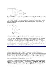


![Microsoft PowerPoint - 05_FTP.ppt [\254\333\256e\274\322\246\241]](https://img.yumpu.com/36298340/1/190x143/microsoft-powerpoint-05-ftpppt-254333256e274322246241.jpg?quality=85)