Adaptive Data Broadcasting in a Mobile Computing Environment

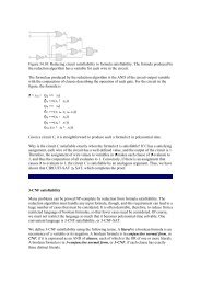
358 W.-C. PENG ET AL.Figure 3. The optimal allocation trees under different times.costs of most levels in the allocation tree to be smaller thanor equal to average cost. Then, for fine tuning, algorithm DLadjusts the data items between neighboring levels with the objectiveof minimizing the total cost of these two neighboringlevels. Note that algorithm DL is greedy in nature and is oftime complexity O(K + n). The algorithmic form of algorithmDL is described below.Algorithm DL.Input: The status table (ST) with K rows, where K is thenumber of broadcast disks in a broadcast disk array.Output: The resulting allocation tree.begin1. for each row i in table ST2. ST(i) · D = ST(i) · C − ST(i) · P ;3. ST(i) · G = false; /* ST(i) · G is the flag for casualchecking*//*Array δ has K − 1 elements which record the costdifference between two neighboring level*/4. for each element i in array δ5. δ[i] =|ST(i) · C − ST(i + 1) · C|6. casual_checking = 0;/*The casual adjustment phase*/7. Choose the row i from table ST such that ST(i) · Dis maximal8. repeat9. begin10. if (i == 1)11. casual_tunning(i, i + 1);12. else if (i == k)13. casual_tunning(i, i − 1);14. else15. {choose the row j where j ∈ (i − 1,i+ 1)such that ST(j) · G is false and δ[j] is maximal;16. casual_tunning(i, j);}17. casual_checking++;18. update table ST and array δ accordingly;19. choose the row i from ST where ST(i) · C is maximaland ST(i) · G is false;20. end21. until casual_checking == K − 1;/*the fine adjustment phase*/22. Construct a priority queue PQ;/*A priority queue is a data structure which returns theelement with the minimal value when one is to removean element from the priority queue*/23. for each element i in array δ24. Insert δ[i] into the PQ;25. while (PQ is not empty)26. begin27. remove the element i from PQ;28. if (ST(i) · C ∑ Ki=1 ST(i) · C/K)move the data item in the rightest side of level i tolevel j and update ST(i) · C accordingly;endelsebeginwhile (ST(i) · C> ∑ Ki=1 ST(i) · C/K)move the data item in the leftest side of level i tolevel j and update ST(i) · C accordingly;end}Table ST (standing for status table) is created to record thecost of each level in the allocation tree, and the number ofrows in table ST is equal to the number of broadcast disks ina broadcast disk array (from line 1 to line 3). Note that in

DYNAMIC LEVELING: ADAPTIVE DATA BROADCASTING 359table ST, thevalueofST(i) · P is the cost of nodes in level ipreviously, whereas the value of ST(i) · C is the cost of nodesin level i when the latest access frequencies were collected.ST(i) · D stores the cost difference associated with level i,i.e., ST(i) · C − ST(i) · P . Also, ST(i) · G is used to indicatewhether the casual tuning is performed or not. Array δhas K − 1 elements that record the cost difference betweentwo neighboring levels (from line 4 to line 5). As can be seenin causal adjustment phase (i.e., from line 7 to line 21), algorithmDL makes sure that most levels of the allocation treesatisfy the requirement of the casual adjustment. Since the casualadjustment intends to let the total cost of allocation treebe evenly allocated to all levels, it is possible that some datanodes would move back and forth between neighboring levels.For execution efficiency, the number of runs for the casualadjustment is limited to be K − 1. Procedure casual_tuningis developed to move data items in level i so as to satisfy thepurpose of the casual adjustment.By exploiting the casual adjustment, data items are roughlyallocated to each level of an allocation tree with the costs ofmost levels are smaller than or equal to average cost. Then,algorithm DL employs the fine adjustment to adjust data itemsbetween neighboring levels. As can be seen from line 22 toline 34 of algorithm DL, neighboring levels are examined onfinding potential movements with the purpose of minimizingthe total cost of neighboring levels. Specifically, in line 27 ofalgorithm DL, the sequence of performing the fine tuning isdetermined by identifying the largest cost difference amongthose between neighboring levels (i.e., the largest value in δ).After identifying the neighboring levels (e.g., level i and leveli + 1) to perform the fine tuning, one should determine thedata movements between these levels. Note that there are twokinds of movements, i.e., pushing up and polling down. Judiciouslyapplying these movements is able to reduce the totalcost of these two neighboring levels. Clearly, if the cost oflevel i is smaller than level i + 1, we should move data itemsfrom level i + 1toleveli and vice versa. After deciding thedirection of data movements, we should determine the numberof data items to move among levels in an allocation tree.Explicitly, we develope procedure push_up and pull_down todetermine such a number. To facilitate the presentation ofalgorithm DL, the procedures of push_up and pull_down aredescribed in detail later. From line 26 to line 34, algorithmDL adjusts data items in neighboring levels iteratively withthe objective of minimizing the total cost of neighboring levelsuntil there is no further adjustment required (i.e., queuePQ is empty). As such, the allocation tree is adjusted so as tominimize the total cost of the allocation tree.Once we identify the direction of data movements to perform,we should determine the number of data items to moveamong levels. Suppose that data items in each level of an allocationtree are sorted according to the descending order of accessfrequencies. In order to evaluate the cost reduction by themovement of pushing up, we have the following definition.Definition 2. Suppose that level i has k − i + 1 nodes,R i ,R i+1 ,...,R k and level i + 1hasj − k data nodes,R k+1 ,R k+2 ,...,R j . The reduction gain achieved by pushingp nodes (i.e., R k+1 ,R k+2 ,...,R k+p )uptoleveli, denotedby u(p), can be formulated as u(p) = (C i,k + C k+1,j ) −(C i,k+p + C k+p+1,j ).In light of definition 2, we devise a procedure push_up toidentify the group of nodes in level i + 1tobemovedupwardto level i so as to maximize the reduction gain betweenthese two neighboring levels. Figure 4 shows the scenario ofpushing up.Procedure push_up(level i, level i + 1){Determine p ∗ such that u(p ∗ ) = max 1pj−k {u(p)};/*determine the maximal value of u(p) when p variesfrom 1 to j − k*/if u(p ∗ )>0push nodes R k+1 ,R k+2 ,...,R k+p ∗ to level i in the tree;elsep ∗ =−1; /*no movement is performed since there isno cost-effective movement*/}Similar to the operation of pushing up, we have definition 3and procedure pull_down below to evaluate the group of nodesin level i to be moved downward to level i + 1 with the purposeof reducing the total cost of these two neighboring levels.Figure 5 illustrates the scenario of pulling down.Definition 3. Suppose that level i has k − i + 1 data nodes,R i ,R i+1 ,...,R k and level i + 1hasj − k data nodes,R k+1 ,R k+2 ,...,R j . The reduction gain achieved by pullingp nodes (i.e., R k−p+1 ,R k−p+2 ,...,R k )downtoleveli + 1,denoted by d(p), can be formulated as d(p) = (C i,k +C k+1,j ) − (C i,k−p + C k−p+1,j ).Figure 4. A scenario of pushing up.Figure 5. A scenario of pulling down.

360 W.-C. PENG ET AL.Table 3The profile of an illustrative example.Time R 1 R 2 R 3 R 4 R 5 R 6 R 7 R 8 R 9 R 10 R 11t 1 0.126 0.123 0.116 0.11 0.1 0.095 0.0869 0.0777 0.0673 0.055 0.0388t 2 0.276 0.239 0.194 0.102 0.08 0.05 0.0298 0.0153 0.0064 0.0019 0.0002Procedure pull_down(level i, level i + 1){Determine p ∗ such that d(p ∗ ) = max 1pk−i+1 {d(p)};/*determine the maximal value of d(p) when p variesfrom 1 to k − i + 1*/if d(p ∗ )>0pull nodes R k−p ∗ +1,R k−p ∗ +2,...,R k down level i + 1in the tree;elsep ∗ =−1; /*no movement is performed since there isno cost-effective movement*/}3.2. An example execution scenario of algorithm DLConsider the profile in table 3 where the number of data itemsn is 11 and the number of broadcast disks is 4. The initial allocationtree is shown in figure 6(a), where the allocation treeis generated according to the access frequencies at t 1 . Thevalues in table ST and their changes made in accordance withthe execution of algorithm DL are shown in table 4. First, algorithmDL chooses the maximal ST(i) · D to start the casualadjustment. In this example, level 1 is chosen since ST(1) · Dis the largest among all levels. As can be seen in table 4(a),since the cost of level 1 is larger than the average cost of alllevels (i.e., ST(1) · C = 0.2575 > ∑ 4i=1 ST(i) · C/4 =(0.2575 + 0.376 + 0.0951 + 0.0085)/4 = 0.184275), dataitems in level 1 should be pulled down to level 2 to meetthe criterion of the casual adjustment. Thus, data item R 2is moved to level 2 and table ST is updated accordingly. Followingthe same procedure, algorithm DL performs procedurecasual_tuning iteratively until casual_checking equalsK − 1(i.e.,4− 1 = 3). Table 4(b) shows the values oftable ST and the corresponding values in array δ after the casualadjustment. The configuration of the allocation tree infigure 6(a) becomes the one shown in figure 6(b). Then, inthe phase of the fine adjustment, each element of array δ withits value is inserted into queue PQ and algorithm DL performsthe fine tuning between neighboring levels. From table 4(b),since δ[3] is the largest, the fine adjustment will be executedbetween level 3 and level 4. As ST(3) · C is smaller thanST(4) · C, those data items in level 4 should be pushed up tolevel 3. It can be verified that data item R 5 should be pushedup to level 3 so as to reduce the total cost of level 3 and level 4.Table 4(c) shows the values of table ST and the correspondingvalues in array δ after the fine tuning is performed betweenlevel 3 and level 4. Figure 6(c) shows the configuration ofthe allocation tree after the first fine tuning. From table 4(c),the next fine tuning is performed between level 2 and level 3.Following the fine adjustment, algorithm DL stops when thereis no further data movement required. Table 4(d) shows theTable 4An execution scenario under algorithm DL. (a) Run 1 of algorithm DL,(b) table ST after the phase of the casual adjustment, (c) table ST after thefirst fine tuning is performed, (d) the final result of table ST.(a)Level i ST(i) · P ST(i) · C ST(i) · D ST(i) · G1 0.1245 0.2575 0.133 ∗ false2 0.326 0.376 0.05 false3 0.25 0.0951 −0.1549 false4 0.1611 0.0085 −0.1526 falseLevel i ST(i) · P ST(i) · C ST(i) · D ST(i) · G δ(b)1 0.1245 0 −0.1245 true 02 0.326 0 −0.326 true 0.1483 0.25 0.148 −0.102 true 0.4028 ∗4 0.1611 0.5508 0.3897 falseLevel i ST(i) · P ST(i) · C ST(i) · D ST(i) · G δ(c)1 0.1245 0 −0.1245 true 02 0.326 0 −0.326 true 0.376 ∗3 0.25 0.376 0.126 true 0.1174 0.1611 0.259 0.0979 false(d)Level i ST(i) · P ST(i) · C ST(i) · D ST(i) · G1 0.1245 0 −0.1245 true2 0.326 0.2165 −0.1095 true3 0.25 0.252 0.002 true4 0.1611 0.1072 −0.0539 falsevalues of table ST after performing algorithm DL. The finalallocation tree is shown in figure 6(d). Note that in this casethe final allocation tree happens to be the optimal one shownin figure 3(c).4. Performance evaluationIn order to evaluate the performance of algorithm DL, wehave implemented a simulation model of the broadcast environment.Specifically, the simulation model is described insection 4.1. Then, we examine the impact of adjusting broadcastprograms in section 4.2. Performance of algorithm DL isanalyzed in section 4.3. In section 4.4, algorithm DL and thework in [14] is comparatively analyzed.4.1. Simulation modelTable 5 summarizes the definitions for some primary simulationparameters. The number of data items to be broadcasted

DYNAMIC LEVELING: ADAPTIVE DATA BROADCASTING 361Figure 6. An execution scenario of algorithm DL: (a)–(c) the adjustment of the allocation tree, and (d) the resulting allocation tree.NotationnKθfno_adjustOPTVF KTable 5The parameters used in the simulation.Definitiontotal number of data items to be broadcastnumber of broadcast disks in a broadcast disk arrayZipf parameterfluctuation factorscheme which does not adjust the broadcast programscheme to generate the optimal broadcast programscheme to generate the broadcast programs staticallyin a broadcast disk array is denoted by n and the number ofbroadcast disks in a broadcast disk array is K. The access frequenciesof broadcast data items are modelled by the Zipf distribution.Let P r (R i ) = ((N − i)/N) θ / ∑ nj=1 ((N − j)/N) θ ,where θ is the parameter of Zipf distribution [5]. It can be verifiedthat the access frequencies become increasingly skewedas the value of θ increases. Specifically, the initial Zipf parameter,denoted by θ 0 , is set to 0.5. θ current is the Zipf parameterfor the current access frequencies, whereas θ previousis the Zipf parameter collected last. The number of f calledthe fluctuation factor is used to determine whether algorithmDL will be executed or not. If the difference between θ currentand θ previous is larger than the value of f , DL will be executedto adjust the broadcast program in order to retain theperformance. For comparison purposes, a scheme, no_adjust,which does not adjust the broadcast program in response tothe change of access frequencies, is implemented. To obtainthe optimal solutions for comparison, we implementedscheme OPT by using the technique of branch and bound[11]. For interest of brevity, the implementation details ofOPT are omitted in this paper. Notice that though schemeOPT is able to find the optimal broadcast program, the executiontime of OPT is prohibitively large due to its exponentialtime complexity. For comparison purposes, we also implementedscheme VF K , which is able to generate broadcastprogram with the number of broadcast disks and the numberof data items given.4.2. The impact of adjusting broadcast programsTo show the advantage of adjusting broadcast programs whenthe access frequencies vary, we set the value of n to 50, thevalue of K to 4 and the value of f to 1. The expected delays ofdata items under no_adjust, DLandOPT are examined withthe value of θ varied. Without loss of generality, assume thatall the data items are of the same size which is used as one unitof waiting time. The initial broadcast program is generated byscheme OPT. The resulting expected delays of data items byrunning no_adjust,DLandOPT are shown in figure 7. It canbe seen from figure 7 that the access frequencies become increasinglyskewed as the value of θ increases and the averageexpected delay of DL decreases since the broadcast programis properly adjusted by DL in accordance with the change ofaccess frequencies of data items. Note that the difference betweenexpected delay of DL and that of no_adjust becomeslarger as the θ increases, indicating the necessity of adjustingbroadcast programs while the access frequencies of dataitems vary. It is worth mentioning that though algorithm DLis applied in 5 times, the expected delays of DL and OPT arestill very close in figure 7, showing the good quality of configurationsadjusted by algorithm DL.

362 W.-C. PENG ET AL.Figure 7. The average expected delays of no_adjust, DLandOPT with thevalue of Zipf parameter varied.Figure 8. The average expected delays of OPT and DL with the value of fvaried.4.3. The performance of algorithm DLWe now investigate the quality of solutions obtained by DLand OPT. Note that algorithm DL will dynamically adjust thebroadcast program while the Zipf parameter varies. In orderto evaluate the impact of increasing the value of f ,wesetthe value of n to 50 and the value of K to 4. Figure 8 showsthe performance results of OPT and DL. As can be seen infigure 8, the difference between expected delay of DL and thatof OPT is almost negligible, showing the very high quality ofthe solutions obtained by algorithm DL. Note that as the valueof f increases, the solutions obtained by algorithm DL are allvery close to the optimal ones, indicating the robustness inalgorithm DL.Next, the experiments of varying the value of K for OPTand DL are conducted where we set the value of n to be 50and the value of f to be 2.5. Figure 9 shows the averageexpected delays of OPT and DL with the value of K varied.As the value of K increases, the expected delays of OPTand DL decrease. This agrees with our intuition since as thenumber of broadcast channels increases, the number of dataitems in each broadcast channel decreases, thereby reducingthe expected delay of data items. Notice that the differencebetween the expected delay of DL and that of OPT is verysmall, again showing the good quality of solutions obtainedby DL. The performance of DL with the value of n varied isexamined where we set the value of K to 5 and the value off to 2.5. The average expected delays of OPT and DL withthe value of n varied are shown in figure 10. As the numberof data items to be broadcast increases, the expected delaysof data items resulted by OPT and DL increase linearly as weanticipate. Also, the difference between the expected delaysresulted by OPT and DL is negligible.4.4. Comparative analysis for VF K and DLIn [14], VF K is designed for the situation where the data accessfrequencies and the number of broadcast channels aregiven. The experimental results show that the broadcast programgenerated by VF K is of very high quality. However,Figure 9. The average expected delays of OPT and DL with the value of Kvaried.Figure 10. The average expected delays of OPT and DL with the value of nvaried.in practice, the data access frequencies may vary as time advances.It is important for broadcast programs to adapt tothe change of the data access frequencies so as to retain theperformance of data broadcasting. In this section, our experimentalresults show that algorithm DL is more efficient toachieve new configuration without re-executing VF K .To evaluate the impact of increasing the value of n, wesetthe value of K to 15 and the value of f to one. Figure 11shows the execution times incurred by VF and DL. In fig-

DYNAMIC LEVELING: ADAPTIVE DATA BROADCASTING 363program generated by VF K will not be adjusted according tothe change of access frequencies. Thus, the performance degradesas the access frequencies vary, justifying the necessityof algorithm DL.5. ConclusionsFigure 11. The execution times incurred by VF K and DL with the value of nvaried.We explored in this paper the problem of adjusting broadcastprograms to cope with the data access frequencies varied. Byexploiting the features of the casual adjustment and the fineadjustment, we developed a heuristic algorithm DL to adjustbroadcast programs when the access frequencies of data itemschange. Performance of algorithm DL was analyzed and asystem simulator was developed to validate our results. Sensitivityanalysis on several parameters, including the numberof data items, the number of broadcast disks, and the variationof access frequencies, was conducted. It was shown byour simulation results that the broadcast programs achievedby algorithm DL are of very high quality and are in fact veryclose to the optimal ones. This feature and the efficiency of algorithmDL justify the practical importance of algorithm DL.ReferencesFigure 12. The execution times incurred by VF K and DL with the value ofK varied.ure 11, the execution times incurred by VF K andbyDLincreaseas the number of data items increases. Note that theexecution time incurred by VF K is larger than that incurredby DL, showing that DL is able to achieve the new configurationmore efficiently when the data access frequencies vary.It is also observed that the curve of VF K in figure 11 is notas smooth as that of DL due to the lack of dynamic allocationadjustment of VF K .Next, we examine the impact of increasing the value of K.Without loss of generality, we set the value of n to 5 and thevalue of f to one. The execution times incurred by VF K andDL with the value of K varied are shown in figure 12. Noticethat when the value of K is smaller than 5, the executiontime incurred by VF K is smaller than that incurred by DL.However, as the value of K increases, the execution time incurredby VF K is significantly larger than that incurred byDL. This indicates that when the value of K increases, theadvantage of algorithm DL over the approach of re-executingalgorithm VF K increases. In all, algorithm DL is able notonly to adjust the broadcast program efficiently in responseto the change of access frequencies of data items but also toproduce the solutions of very high quality. Note that the capabilityof adjusting broadcast programs dynamically should beviewed as an enhanced feature rather than a limitation. In fact,when the value of f is set to be infinite, the initial broadcast[1] S. Acharya, R. Alonso, M. Franklin and S. Zdonik, Broadcast disks:Data management for asymmetric communication environments, in:Proceedings of ACM SIGMOD (March 1995) pp. 199–210.[2] D. Barbara, Mobile computing and databases – a survey, IEEE Transactionson Knowledge and Data Engineering 11(1) (January/February1999) 108–117.[3] M.-S. Chen, P.S. Yu and K.-L. Wu, Indexed sequential data broadcastingin wireless mobile computing, in: 17th IEEE International Conferenceon Distributed Computing Systems (1997) pp. 124–131.[4] M.H. Dunham, Mobile computing and databases, Tutorial of InternationalConference on Data Engineering (February 1998).[5] J. Gray, P. Sundaresan, S. Englert, K. Baclawski and P. J. Weinberger,Quickly generating billion-record synthetic databases, in: Proceedingsof ACM SIGMOD ( March 1994) pp. 243–252.[6] Q.L. Hu, D.L. Lee and W.-C. Lee, Dynamic data delivery in wirelesscommunication environments, in: Proceedings of International Workshopon Mobile Data Access (November 1998) pp. 218–229.[7] Q. Hu, D.L. Lee and W.-C. Lee, Performance evaluation of a wirelesshierarchical data dissemination system, in: Proceedings of the Fifth AnnualInternational Conference on Mobile Computing and Networking(1999) pp. 163–173.[8] Q. Hu, W.-C. Lee and D.L. Lee, Indexing techniques for wireless databroadcast under data clustering and scheduling, in: Proceedings of theEighth International Conference on Information and Knowledge Management(November 1999) pp. 351–358.[9] T. Imielinski, S. Viswanathan and B. Badrinath, Data on air: organizationand access, IEEE Transactions on Knowledge and Data Engineering9(3) (June 1997) 353–372.[10] J. Jing, A. Helal and A. Elmagarmid, Client–server computing in mobileenvironments, ACM Computing Surveys 31(2) (June 1999) 117–157.[11] R.C.T. Lee, R.C. Chang, S.S. Tseng and Y.T. Tsai, Introduction to theDesign and Analysis of Algorithms (Unalis Press).[12] W.-C. Lee and D.-L. Lee, Signature caching techniques for informationfiltering in mobile enviroments, ACM Journal of Wireless Networks5(l) (January 1999) 57–67.

364 W.-C. PENG ET AL.[13] S.-C. Lo and A.L.P. Chen, Optimal index and data allocation in multiplebroadcast channels, in: Proceedings of the 16th International Conferenceon Data Engineering (March 2000) pp. 293–302.[14] W.-C. Peng and M.-S. Chen, Dynamic generation of data broadcastingprograms for a broadcast disk array in a mobile computing environment,in: Proceedings of the ACM 9th International Conference onInformation and Knowledge Management (November 2000) pp. 38–45.[15] E. Pitoura and P.K. Chrysanthis, Exploiting versions for handling updatesin broadcast disks, in: Proceedings of 25th International Conferenceon Very Large Data Bases (September 1999) pp. 114–125.[16] K. Prabhakara, K.A. Hua, and J.-H. Oh, Multi-level multi-channel aircache designs for broadcasting in a mobile environment, in: Proceedingsof the 16th International Conference on Data Engineering (February2000) pp. 167–176.[17] N. Shivakumar and S. Venkatasubramanian, Energy efficient indexingfor information dissemination in wireless systems, ACM Journal ofWireless Networks and Applications 1(4) (January 1996) 433–446.[18] K. Stathatos, N. Roussopoulos and J.S. Baras, Adaptive data broadcastin hybrid networks, in: Proceedings of the 23rd International Conferenceon Vary Large Data Bases (August 1997) pp. 326–335.[19] C.-J. Su and L. Tassiulas, Broadcast scheduling for information distribution,in: Proceedings of the 6th IEEE International Conference onInformation and Communication (April 1997) pp. 109–117.[20] C.-J. Su and L. Tassiulas, Joint broadcast scheduling and user’s cachemanagement for efficient information delivery, in: Proceedings of the4th ACM/IEEE International Conference on Mobile Computing andNetworking (October 1998) pp. 33–42.[21] WAP application in Nokia, http://www.nokia.com/corporate/wap/future.html[22] WAP application in Unwired Planet, Inc., http://phone.com[23] J.X. Yu, T. Sakata and K. Tan, Statistical estimation of access frequenciesin data broadcasting environments, ACM/Baltzer Wireless Networks6(2) (March 2000) 89–98.Wen-Chih Peng biography and photo not available at time of publication.E-mail: wcpeng@arbor.ee.ntu.edu.twJiun-Long Huang biography and photo not available at time of publication.E-mail: jlhuang@arbor.ee.ntu.edu.twMing-Syan Chen biography and photo not available at time of publication.E-mail: mschen@cc.ee.ntu.edu.tw