Mirror MoCap: Automatic and efficient capture of dense 3D facial ...

Visual Comput (2005) 

DOI 10.1007/s00371-005-0291-5 ORIGINAL ARTICLE 

I-Chen Lin (✉) 

Ming Ouhyoung 

Mirror MoCap: Automatic and efficient 

capture of dense 3D facial motion parameters 

from video 

Published online: 9 June 2005 

© Springer-Verlag 2005 

I-C. Lin 

Dept. of Computer and Information 

Science, National Chiao Tung University, 

1001 Ta Hsueh Road, Hsinchu, 300, 

Taiwan 

e-mail: ichenlin@cis.nctu.edu.tw 

M. Ouhyoung 

Dept. of Computer Science and 

Information Engineering, National Taiwan 

University, No.1 Roosevelt Rd. Sec. 4, 

Taipei, 106, Taiwan 

e-mail: ming@csie.ntu.edu.tw 

Abstract In this paper, we present 

an automatic and efficient approach 

to the capture of dense facial motion 

parameters, which extends our previous 

work of 3D reconstruction from 

mirror-reflected multiview video. 

To narrow search space and rapidly 

generate 3D candidate position lists, 

we apply mirrored-epipolar bands. 

For automatic tracking, we utilize 

spatial proximity of facial surfaces 

and temporal coherence to find the 

best trajectories and rectify statuses 

of missing and false tracking. 

More than 300 markers on a subject’s 

face are tracked from video at a process 

speed of 9.2 frames per second 

(fps) on a regular PC. The estimated 

3D facial motion trajectories have 

been applied to our facial animation 

system and can be used for facial 

motion analysis. 

Keywords Facial animation · Motion 

capture · Facial animation 

parameters · Automatic tracking 

1 Introduction 

From a big smile to a subtle frown to a pursed mouth, 

a face can perform various kinds of expressions to implicitly 

reveal one’s emotions and meanings. However, these 

frequent expressions, which we usually take for granted, 

involve highly complex internal kinematics and sophisticated 

variations in appearance. For example, during pronunciation, 

nonlinear transitions of a face surface depend 

on preceding and successive articulations, a phenomenon 

known as coarticulation effects [10]. 

In order to comprehend the complicated variations 

of a face, recently more and more researchers have been 

using motion capture techniques that simultaneously 

record 3D motion of a large number of sensors. When 

sensors are placed on a subject’s face, these techniques 

can extract the approximate motion of these designated 

points. Today, commercial motion capture devices, such 

as optical or optoelectronic systems, are able to accurately 

track dozens of sensors on a face. However, these devices 

are usually very expensive, and the expense becomes 

a significant barrier for researchers intending to devote 

themselves to areas related to facial analysis. Moreover, 

current motion capture devices are unable to track spatially 

dense facial sensors without interference. Not only 

can a large quantity of facial motion parameters directly 

provide more realistic surface deformation for facial animation, 

but the dense facial motion data could also be 

a key catalyst for further research. From the aspect of face 

synthesis, in the current process of animation production, 

facial motion capture data of 20 to 30 feature points are 

used to drive a well-prepared synthetic head. Motion vectors 

on the face’s uncovered areas are estimated by internal 

virtual muscles, scattering functions, or surface patches. 

Animators can only adjust coefficients of the muscles or 

patches empirically from their observations. With dense 

facial motion data as criteria, the coefficients can be automatically 

calculated, and the results will be more faithful 

to real human facial expression. Regarding facial analysis, 

numerous hypotheses or models have been proposed 

to simulate facial motion and kinematics. Most current research 

uses only sparse facial feature points [18, 19] due to 

tracking device capacities. Sizeable and dense facial mo-

I-C. Lin, M. Ouhyoung 

tion trajectories can provide further detailed information 

for correlations of facial surface points in visual speech 

analysis. 

In our previous work [20], we proposed an accurate 3D 

reconstruction algorithm for mirror-reflected multiview 

images and a semiautomatic 3D facial motion tracking 

procedure. Our previous system can track around 50 facial 

markers using a single video camcorder with two mirrors 

under normal light conditions. When tracking dense facial 

markers, we found that ambiguity in block matching 

caused the tracking to degenerate dramatically. Occlusion 

is the most critical problem: for example, when our 

mouths are pouting or opened wide, the markers below the 

lower lips vanish in video clips. We tried to use thresholding 

in block matching and Kalman predictors to tackle this 

problem; despite our efforts, it works satisfactorily only 

for short-term marker occlusion. 

Fully automatic tracking of multiple target trajectories 

over time is called the “multitarget tracking problem” 

in radar surveillance systems [8]. When only affected 

by measurement error and false detection, this 

problem is equivalent to the minimum cost network flow 

(MCNF) problem. The optimal solution is efficient [9, 27]. 

Nevertheless, when measurement errors, missing detection 

(false negative), and false alarms (false positive) all 

occur during tracking, time-consuming dynamic programming 

is required to estimate approximate trajectories, and 

the tracking results can degenerate seriously even if the 

occurrence frequency of missing detection slightly increases 

[28]. In our experiments, even though fluorescent 

markers and blacklight lamps are used to enhance the clarity 

of markers and to improve the steadiness of markers’ 

projected colors, missing and false detections are still unavoidable 

in the feature extracting process. 

Fortunately, the motion of markers on a facial surface 

is unlike that of targets tracked in radar systems. Targets 

in the general multitarget-tracking problem move independently, 

and consequently the judgement of a target’s best 

trajectory can only stand on its prior trajectory. In contrast, 

points on a facial surface have not only temporal continuity 

but also spatial coherence. Except for the mouth, 

nostrils, and eyelids, a face is mostly a continuous surface, 

and a facial point’s positions and movements are similar 

to those of its neighbors. With this additional property, automatic 

diagnoses of missing and false detection become 

feasible and the computation is more efficient. 

Guenter et al. [14] tracked 182 dot markers painted 

with fluorescent pigments for near-UV light. This research 

used special markers and lights to enhance the feature detection, 

and the researchers took into account the spatial 

and temporal consistency for reliable tracking. Guenter 

and his colleagues’ impressive work inspired us. 

In this proposed work, we follow our previous framework 

of estimating 3D positions from mirror-reflected 

multiview video clips [20] in which two mirrors are placed 

near a subject’s face and a single video camera is used 

to record simultaneously frontal and mirrored facial images. 

Instead of normal light conditions, to improve clarity, 

we also apply markers with UV-responsive pigments 

for blacklight blue (BLB) fluorescent lights. Compared to 

Guenter et al.’s work, the proposed method is more efficient 

and versatile. 

Guenter et al.’s work required subjects’ heads to be 

immobile because of the limitation of markers’ vertical 

orders in their marker matching routine, and therefore 

head movement had to be tracked independently by other 

devices. In addition, there was no explicit definition of 

tracking errors in this method, and an iterative approach 

was used for node matching. In contrast, our proposed 

method is capable of automatically tracking both facial expressions 

and head motions simultaneously without synchronization 

problems. Furthermore, we propose using 

mirrored epipolar bands to rapidly generate 3D candidate 

points from projections of extracted markers and forming 

the tracking as a node-connection problem. Both spatial 

and temporal coherence of dense markers’ motion are applied 

to efficiently detect and compensate missing tracking, 

false tracking, and tracking conflicts. Our system is 

now able to capture more than 300 markers at a process 

speed of 9.2 fps and can be extended for a regular PC to 

track more than 100 markers from live video in real time. 

This paper is organized as follows. In Sect. 2, we mention 

related research in facial motion capture and face 

synthesis. Section 3 describes equipment setting and gives 

an overview of our proposed tracking procedure. Section 4 

presents how to extract feature points from image sequences 

and explains the construction of 3D candidates. In 

Sect. 5, we present a procedure to find the best trajectories 

and to tackle the problem of missing and false tracking. 

The experimental results and discussion are presented in 

Sect. 6. Finally, we present our conclusions in Sect. 7. 

2 Related work 

For tracking to be fully automatic, some studies have employed 

a generic facial motion model. Goto et al. [13] 

used separate simple tracking rules for eyes, lips, and 

other facial features. Pighin et al. [23, 24] proposed tracking 

animation-purposed facial motion based on linear 

combination of 3D face model bases. Ahlberg [1] proposed 

a near-real-time face tracking system without markers 

or initialization. In “voice puppetry” [7], Brand applied 

a generic head mesh with 26 feature points, where 

spring tensions were assigned to each edge connection. 

Such a generic facial motion model can rectify “derailing” 

trajectories and is beneficial for sparse feature tracking; 

however, an approximate model can also overrestrict the 

feature tracking while a subject does exaggerated or unusual 

facial expressions.

Mirror MoCap: Automatic and efficient capture of dense 3D facial motion parameters from video 

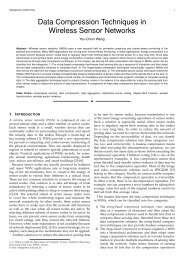
Fig. 1. Applying extracted motion parameters of 300 markers to a sythetic face. The first row is extracted 3D motion vectors where the 

line segments represent displacement comparing to the neutral face; the middle row is a generic head driven by retargeting motion data; 

in the third row, the retargeting motion data are applied to a personalized face 

For 3D facial motion tracking from multiple cameras, 

an optoelectronic system, e.g., Optotrak (www.ndigital 

.com/optotrak.html), uses optoelectronic cameras 

to track infrared-emitting photodiodes on a subject’s face. 

This kind of instrument is highly accurate and appropriate 

for analysis of facial biomechanics or coarticulation effects. 

However, each diode needs to be powered by wires, 

which may interfere with a subject’s facial motion. 

Applying passive markers can avoid this problem. 

In the computer graphics industry for movies or video 

games, animators usually make use of protruding spherical 

markers with high response to a special spectrum 

band, e.g., red visible light or infrared in the vicon series 

(www.vicon.com). The high response and spherical 

shape make feature extraction and shape analysis easier, 

but these markers do not work well for lip surface 

motion tracking because people sometimes tuck in their 

lips, and these markers will obstruct the motion. Besides, 

the extracted motion of protruding markers is not the exact 

motion on a face surface but the motion at a small distance 

above the surface. 

In addition to capturing stereo videos with multiple 

cameras, Patterson et al. [22] proposed using mirrors 

to acquire multiple views for facial motion recording. 

They simplified the 3D reconstruction problem and assumed 

mirrors and the camera were vertical. Basu et 

al. [3] employed a front view and a mirrored view to 

capture 3D lip motion. In our previous work [20], we 

also applied mirrors for acquirement of facial images 

with different view directions. However, our 3D reconstruction 

algorithm proved simpler yet more accurate 

because it conveniently uses symmetric properties of mir-


rored objects. Readers can refer to [20] for a detailed 

explanation. 

Some devices and research apply other concepts to 

estimate 3D motion or structure. Blanz et al. [6] used 

the optical flow method for correspondence recovery between 

scanned facial keyframes. Structured-light-based 

systems [11, 17, 29] project patterns onto a face and can 

therefore extract 3D shape and texture. Detailed undulation 

on a face surface can be captured with high-resolution 

cameras. Zhang et al.’s system [29] can even automatically 

track correspondences from consecutive depth images 

without markers by template matching and optical 

flow. However, the estimation can be unreliable for textureless 

regions. 

3 Overview 

3.1 Equipment setting 

In order to enhance the distinctness of markers from others 

in video clips, we utilize the fluorescent phenomenon 

covering markers with fluorescent pigments. When illuminated 

by BLB lamps, the pigments are excited and 

emit fluorescence. Since the fluorescence belongs to visible 

light, no special attachment lens is required for the 

video camera. In our experiments, we found that fluorescent 

colors of our pigments could be roughly divided 

into four classes, green, blue, pink, and purple. To avoid 

ambiguity in the following tracking, we evenly place 

four classes of markers on a subject’s face and keep 

markers as far as possible from those of the same color 

class. 

The equipment setting of our tracking system is shown 

in Fig. 2. Two mirrors and two BLB lamps are placed in 

front of a digital video (DV) camcorder. The orientations 

and locations of mirrors can be arbitrary, as long as the 

front- and side-view images of a subject’s face are covered 

by the camera’s field of view (Fig. 3). 

After confirming the camera’s view field, including 

the frontal and two side views, the mirrors, the camera, 

and the intrinsic parameters of the camera have 

to be fixed. We use Bouguet’s camera calibration 

toolbox (www.vision.caltech.edu/bouguetj/ 

calib_doc) based on Heikkila et al.’s work [16] to 

evaluate the intrinsic parameters (including focal lengths, 

distortion, etc.). The coordinate system is then normalized 

and undistorted based on the intrinsic parameters, called 

the normalized camera model. After this, we estimate the 

mirrors’ parameters by our previous work [20]. The normalized 

coordinate system is applied to all the following 

steps. 

Fig. 2. The tracking equipment. This photo is taken under normal light. Two “Blacklight Blue”(BLB) lamps are placed in front of a subject 

and mirrors. The low-cost special lamps are coated with fluorescent powders, and it can emit long wave UV-A radiation to excite 

luminescence


Fig. 3. A captured video clip of fluorescent markers illuminated only by BLB lamps. The fluorescence is visible in the visible light 

spectrum and no special lens is required for filtering 

3.2 Initialization 

Initialization of the tracking procedure reconstructs the 

3D positions of markers in the first frame (the neutral 

face). To efficiently recover point correspondences in the 

first frame, two approaches can be used for different 

conditions. 

The first approach is to employ 3D range scanned 

data. Figure 4 shows the process of recovering point correspondences. 

Before applying 3D scanned data, the coordinate 

system of the data must conform to the normalized 

camera model. First, markers’ projected positions are extracted 

(Fig. 4a), and then a user has to manually select n 

(n > 3) corresponding point pairs on the nose tip, eye corners, 

mouth corners, etc. in the first video clip to form a 

3D point set S a . After corresponding feature points in 3D 

scanned data, S b , are also designated, the affine transformation 

between 3D scanned data and specified markers’ 3D 

structure can be evaluated by a least-squares solution proposed 

by Arun et al. [2]. 

While we extend the vector −→ op i ,whereo is the camera’s 

lens center and p i the extracted projected position 

of marker i in the frontal view, the intersection of the 

line −→ op i and 3D scanned data is regarded as the 3D position 

of marker i, denoted as m i . The corresponding point 

p ′ i 

in a side view is then recovered by mirroring m i to 

Fig. 4. Recovering 2D point correspondences with 3D scanned data and RBF interpolation


the mirrored space and projecting the mirrored one, m ′ i , 

back to the image plane. Due to perturbation of measurement 

noise, within a tolerant region the nearest point 

of the same color class is regarded as the corresponding 

point p ′ i . 

The other approach is to recover point correspondences 

by evaluating a subject’s 3D face structure directly from 

rigid-body motion. If an object is rigid or not deformable, 

affine transformation (rotation R and translation t) resulting 

from motion is equivalent to the inversed affine 

transformation resulting from changes in the coordinate 

system. Therefore, reconstructing the 3D structure from 

rigid-body motion is equivalent to reconstructing the 3D 

structure from multiple views [26]. A subject is required 

to retain his or her face in a neutral expression and slowly 

move his or her head in four directions: right-up, rightdown, 

left-up, and left-down. A preliminary 3D structure 

of the face can be estimated from markers’ projected motion 

in the frontal view, and point correspondence can then 

be recovered. 

3.3 Overview of the tracking procedure 

Figure 5 is the flow chart of the proposed tracking procedure. 

As mentioned in the Sect. 3.1, in the first step, we have 

to evaluate the parameters of the video camera and two 

mirrors. Markers’ 3D positions in the neutral face are then 

estimated by the methods introduced in Sect. 3.2. 

For each successive frame t (t = 2 ...T end ), feature 

extraction is first applied to extract markers’ projected 

positions in the frontal and mirrored views. From the projected 

2D positions in real-mirrored image pairs and mirror 

parameters, we can calculate a set of 3D positions, 

which are the markers’ possible 3D positions. We call 

these 3D positions “potential 3D candidates” (Fig. 8). 

After this step, the tracking becomes a node-connection 

problem with the possibility of missing nodes. 

Since we allow a subject’s head to move naturally, we 

find that the head movement dominates the markers’ motion 

trajectories. To avoid head motion seriously affecting 

the tracking results, before the “node matching” the global 

Fig. 5. The flow chart of our automatic 3D motion tracking procedure for dense UV-responsive markers


head motion has to be estimated and removed from 3D 

candidates. The head motion is estimated from a set of 

special markers, and adaptive Kalman filters, which work 

according to previous head motion transition, are applied 

to improve the stability. 

After the head motion is removed from the 3D candidates, 

for each marker we take into account its previous 

trajectories and its neighbors’ motion distribution to 

judge whether there is a most appropriate candidate or it is 

a missing-node situation. Once a marker belongs to a situation 

of missing node, false tracking, or tracking conflict, 

we apply the comprehensive information of spatial and 

temporal coherence to estimate the actual motion. Again, 

for each marker an individual Kalman filter is applied to 

improve the tracking stability. 

Details of feature extraction and the generation of 3D 

candidates are described in Sect. 4. The tracking issues 

about head motion estimation, finding 3D point correspondences, 

and detection and rectification of tracking errors 

are then presented in Sect. 5. 

4 Constructing 3D candidates from video clips 

For efficiency of tracking, we first have to narrow the 

search space. This issue can be divided into two parts: extracting 

markers’ projected 2D positions and constructing 

potential 3D candidates. 

4.1 Extracting markers from video clips 

As shown in the video clip (Fig. 3), because we use 

UV-responsive pigments and BLB lamps, markers are 

conspicuous in video clips. Hence, the automatic feature 

extraction can be more reliable and more feasible 

than under normal light conditions. We mainly follow the 

methodology of connected component analysis in computer 

vision, which is composed of thresholding, connected 

component labeling, and region property measurement, 

but we also slightly modify the implementation for 

computational efficiency. 

Since the intensity of UV-responsive markers is much 

higher than that of other markers, to exclude pixels that 

have less probability of marker projection, the first stage 

is color thresholding. For efficiency, we skip the mathematical 

morphology operations used by many feature extraction 

systems. The thresholding works satisfactorily in 

most cases; the most troublesome case, interlaced scan 

lines, can be solved more efficiently by merging nearby 

connected components. 

The second stage is color labeling. In our experiment, 

we collect six kinds of UV-responsive markers that 

are painted with pink, yellow, green, white, blue, and 

purple pigments. However, when illuminated by BLB 

lamps, there are only four typical colors—pink, bluegreen, 

dark blue, and purple. Hence, we mainly categorize 

markers into four color classes and each color 

class comprises dozens of color samples. A selection tool 

is provided to select these color samples from training 

videos. To classify the color of a pixel in video clips, the 

nearest neighborhood method (1-NN) is applied. To reduce 

the classification error resulting from intensity variation, 

the matching operation works on a normalized color 

R 

space (nR, nG, nB), wherenR = √ , nG = 

(R 2 +G 2 +B 2 ) 

G 

√ 

(R 2 +G 2 +B 2 ) , nB = 

√ 

B 

,and(R, G, B) is the 

(R 2 +G 2 +B 2 ) 

original color value. In general, the more color samples 

in a color class, the more accurate the color classification 

of a pixel. For real-time or near-real-time applications, 

around four color samples in each color class are sufficient. 

Connected component labeling is the third stage 

in our feature extraction. It groups connected pixels 

with the same color label number as a component, and 

we adopt 8-connected neighbors. In our case, a marker’s 

projection is smaller than a radius of five pixels, 

and thus the process of connected component labeling 

can be simplified much more than general connectedcomponent-labeling 

approaches. We modify the classical 

algorithm [15] as partial connected component labeling 

(PCCL). Unlike the classical algorithm, for each pixel 

(i, j) we take a one-pass process and check only its preceding 

neighbors, (i − 1, j − 1), (i, j − 1), (i + 1, j − 1), 

and (i − 1, j). Not all 8-connected components can be labeled 

as the same group by PCCL since we do not use 

a large equivalent class table for transiting label numbers 

as in the classical one. But the problem of inconsistent 

label numbers can easily be solved in our next 

stage. 

After the process of partial connected component labeling, 

there are still redundant connected components 

caused by interlaced fields of video, incomplete connected 

component labeling, or noise. The fourth stage is to refine 

the connected components to make extracted components 

as close as possible to the actual markers’ projection. Because 

markers are placed evenly on a face and the shortest 

distance between two markers of the same color class 

is longer than the diameter of a dot marker, nearby connected 

components should belong to the same marker. 

Therefore, the first two kinds of redundant connected components 

can be simply tackled by merging components 

with a distance less than the markers’ average diameter. 

For the redundant components caused by noise, we suppress 

them by removing connected components less than 

four pixels. 

4.2 Constructing 3D candidates by mirrored epipolar 

bands 

If there are N f and N s feature points of a certain color 

class extracted in the frontal and side views respectively,


each point corresponding pair can generate a 3D candidate, 

and therefore there are a total of N f N s 3D candidates 

of this color class. Guenter et al. [14] took all N f N s potential 

3D candidates to track N mrk markers’ motion, where 

N mrk is the amount of actual markers, N mrk ≪ N f N s . 

However, in a two-view system, given a point p i in the 

first image, its corresponding point is constrained to lie on 

a line called the “epipolar line” of p i . With this constraint, 

one only has to search features along the epipolar line. The 

number of 3D candidates decreases substantially and the 

computation is much more efficient. 

We found that there is a similar constraint in our 

mirror-reflected multiview structure. Since a mirrored 

view can be regarded as a flipped view from a virtual 

camera, the constraint should also exist but be flipped. 

We call this mirrored constraint the “mirrored epipolar 

line.” We briefly introduce the concept of the mirrored 

epipolar line in Fig. 6. We assume that p is an 

extracted feature point, o the optic center, and p ′ the un- 

known corresponding point in the mirrored view. Since 

p is a projection, the actual marker’s 3D position, m, 

must lie on the line l op . According to the mirror symmetry 

property, the mirrored marker’s 3D position, m ′ , 

must lie on l ′ op , which is a symmetric line of l op with respect 

to the mirror plane. When a finite-size mirror model 

is adopted, the projection of l ′ op is a line segment, and 

we denote it as p ′ a p′ b . The corresponding point p′ must 

then lie on this mirrored epipolar line segment p ′ a p′ b ,or 

otherwise the marker m is not visible in the mirrored 

view. 

The mirrored epipolar line of a point p can easily 

be evaluated. In our previous work [20], we deduced an 

equation between point p, p ′ and a mirror’s normal u = 

[a, b, c] T : 

(p ′ ) T Up= 0, where U = 

[ 0 −c 

] b 

c 0 −a . (1) 

−b a 0 

After we expand p and p ′ by their x, y, andz components, 

the equation becomes 

[ x 

′ 

p y ′ p 1 ] [ ] 

−cy p + b 

cx p − a = 0 , (2) 

−bx p + ay p 

and the line 

(−cy p + b)x ′ p + (cx p − a)y ′ p + (−bx p + ay p ) = 0 (3) 

is the mirrored epipolar line of p. 

For noise tolerance capability during potential 3D candidate 

evaluation, we extend the line k pixels up and down 

(k = 1.5 in our case) to form a “mirrored epipolar band” 

and search corresponding points of the same color class 

within the region between two constraint lines 

(−cy p + b)x ′ p + (cx p − a)y ′ p + (−bx p + ay p ) 

+ (cx p − a)k = 0 (3a) 

and 

(−cy p + b)x ′ p + (cx p − a)y ′ p + (−bx p + ay p ) 

− (cx p − a)k = 0 . 

(3b) 

Fig. 6. A conceptual diagram of the mirrored epipolar line. p is an 

extracted feature in the frontal view and l op is the line across o and 

p. l ′ op is the line symmetric to l op by the mirror plane. m a m b is 

the projection segment of l ′ op on the mirror plane. p′ a p′ b 

, the projection 

of m a m b on the image plane I, is the mirrored epipolar line 

segment of p 

Figure 7 shows an example of potential point corresponding 

pairs generated by the mirrored epipolar constraint; 

Fig. 8 shows the 3D candidates generated from the constrained 

point correspondences. 

With this step the following tracking procedure can focus 

mainly on the set of potential 3D candidates. However, 

because there is measurement noise in extracted connected 

components and some markers are even occluded, the 3D 

candidates may not include all markers’ positions. Therefore, 

an error-tolerant procedure has to be used for automatic 

tracking.


Fig. 7. Candidates of point corresponding pairs under mirrored epipolar constraints. For each extracted feature in the frontal view, each 

feature point of the same color that lies within its mirrored epipolar band is regarded as a corresponding point 

Fig. 8. Potential 3D candidates generated under the mirrored epipolar constraint and the distance constraint. 3D candidates are first constructed 

from candidates of point correspondences; those whose positions are out of a bounding box are removed from the list of potential 

candidates 

5 Reliable tracking 

The 3D motion trajectories of markers comprise both facial 

motion and head motion. Because the moving range of 

a head is larger than that of facial muscles, when a subject 

enacts facial expressions and moves his or her head at the 

same time, most of the markers’ motion results from head 

motion. This situation could result in the Kalman predictors 

and filters affected mainly by head motion. We adopt 

separate Kalman predictors/filters for head motion and facial 

motion tracking, and we find that the detection and 

rectification of tracking error are more reliable if head motion 

is removed in advance. 

5.1 Head movement estimation and removal 

We assume the head pose in the first frame (t = 1) is upright. 

We also define the head motion at time t as the affine 

transformation of the head pose at time t with respect to 

the head pose at t = 1. The relation can be represented as 

h(t) = R head (t) · h(1) + T head (t), (4) 

where h can be any point on a head irrelevant to facial motion, 

R head (t) is rotation, and T head (t) is translation. For 

automatic head movement tracking, seven specific markers 

are pasted on locations invariant to facial motion, such 

as a subject’s ears and the concave tip on the nose column.


Adaptive Kalman filters are used to alleviate unevenness 

in trajectories resulting from measurement errors. 

R head (t) and T head (t) both have three degrees of freedom. 

T head (t) =[t x (t), t y (t), t z (t)] T . R head (t) is a 3×3matrix 

and can be parameterized in terms of (r x (t), r y (t),and 

r z (t)) in radians. Through least-squares fitting methods 

comparing elements of Eq. 5, (r x (t), r y (t), andr z (t)) can 

be extracted from R head (t). 

R head = R z R y R x 

= 

= 

[ cos(rz ) 

][ ][ ] 

− sin(r z ) 0 cos(rr ) 0 sin(r y ) 1 0 0 

sin(r z ) cos(r z ) 0 0 1 0 0 cos(r x ) − sin(r x ) 

0 0 1 − sin(r y ) 0 cos(r r ) 0 sin(r x ) cos(r x ) 

[ c(rz )c(r y ) −s(r z )c(r x ) + c(r z )s(r y )s(r x ) s(r z )s(r x ) + c(r z )s(r y )s(r x ) 

s(r z )s(r y ) c(r z )c(r x ) + s(r z )s(r y )s(r x ) −c(r z )s(r x ) + s(r z )s(r y )s(r x ) 

−s(r y ) c(r y )s(r x ) c(r y )c(r x ) 

where R z , R y ,andR x are rotation matrices along the z-, 

y-, and x-axes; c() and s() are abbreviations of cos() and 

sin(). Kalman filters are applied directly to these six parameters: 

[r x (t), r y (t), r z (t), t x (t), t y (t), t z (t)]. The process 

of head motion evaluation is as follows. We use r x (t +1|t) 

to represent the prediction of parameter r x at time t + 1 

based on previous data of r x (1) to r x (t); similarly for other 

parameters. 

Step 1. Designate specific markers s i (for i = 1 ...N smrk , 

where N smrk is the amount of specific markers, 

N smrk = 7 in our case) for head motion tracking 

from the reconstructed 3D markers of the neutral 

face (t = 1), and denote their positions as 

ms i (1). (Either a specific color is used for the special 

markers or users have to designate them in the 

first frame.) 

Step 2. Initialize parameters of adaptive Kalman filters 

and set r x (1) = r y (1) = r z (1) = 0, t x (1) = t y (1) = 

t z (1) = 0, and t = 1. 

Step 3. Predict the head motion parameters r x (t + 1|t), 

r y (t + 1|t), r z (t + 1|t), t x (t + 1|t), t y (t + 1|t), and 

t z (t + 1|t) by Kalman predictors and then construct 

R head (t + 1|t) and T head (t + 1|t) by Eq. 5. 

Increase timestamp t = t + 1 

Step 4. Generate predicted positions of specific markers 

as 

] 

(5) 

ms i (t|t − 1) = R head (t|t − 1) × ms i (1) 

+ T head (t|t − 1) (6) 

and find ms i (t) by searching the nearest potential 

3D candidates of the same color. The search is restricted 

within a distance d srch from ms i (t|t − 1). 

If no candidate is found, set the marker as invalid 

at time t. 

Step 5. Detect tracking error: if estimated motions are abnormal 

when compared to other specific markers, 

then set the markers of odd estimation as invalid at 

time t. 

(The tracking error detection is presented in the 

next subsection; we skip the details here.) 

Step 6. Estimate the affine transformation (R msr and 

T msr ) of valid specific markers between time t and 

the first frame by the method proposed by Arun et 

al. [2]. 

Step 7. Extract r msr_x (t), r msr_y (t), and r msr_z (t) from 

R msr by Eq. 5 and extract t msr_x (t), t msr_y (t), and 

t msr_z (t) from T msr . 

Take the extracted parameters as measurement inputs 

to the adaptive Kalman filter and estimate the 

output [r x (t), r y (t), r z (t), t x (t), t y (t), t z (t)]. 

Step 7. Ift > T limit , stop; else go to Step 3. 

We use a position-velocity configuration for the Kalman 

filters for translation, where 3D positions are measurement 

input and the internal states are positions and velocities. 

The operation of the Kalman filters for rotation is similar, 

but the input is a set of angles and the internal states represent 

angles and angular velocities. Once the head motion 

at time t is evaluated, an inverse affine transformation is 

applied to all 3D candidates for head motion removal. 

5.2 Recovering frame-to-frame 3D point correspondence 

with outlier detection 

In this subsection, we assume that head motion is removed 

from potential 3D candidates, and our goal is to 

track markers’ motion trajectories from a frame-by-frame 

sequence of potential 3D candidates. Figure 9 is a conceptual 

diagram of the problem statement. For clarity of 

explanation, we take the situation of only one color class 

of markers as examples. The methodology of processing 

each color class independently can extend to cases of multiple 

color classes. 

The number of potential 3D candidates in a frame is 

around 1.2 ∼ 2.3 times the number of the actual markers. 

The additional 3D candidates can be regarded as false detection 

in the multitarget tracking problem. If only false 

detection occurs, the graph algorithms for minimum cost 

network flow (MCNF) can evaluate the optimal solution. 

In our case, we employ Kalman predictors and filters to 

efficiently calculate the time-varying position variation of 

each marker. However, a marker can “miss” in video clips 

occasionally. The missing condition results from blocking 

or occlusion due to camera views, incorrect classification 

of marker colors, or noise disturbance. When the missing 

and false detection occur concurrently, a simple tracking 

method without evaluation of tracking error would degenerate 

and the successive motion trajectories could be 

disordered. 

We use an example to explain the serious consequence 

of tracking errors. In Fig. 10, marker B is not included 

in the potential 3D candidates of the third frame, and its 

actual position is denoted as B(3). Based on the previous 

trajectory, B’(3) is the nearest potential candidate with


Fig. 9. A conceptual figure for the problem statement of 3D marker tracking. The markers’ 3D positions in the 1st frame are first evaluated. 

The goal of 3D motion tracking is to find frame-to-frame 3D point correspondences from sequences of potential 3D candidates 

Fig. 10. An example of tracking errors resulting from missing markers 

respect to the predicted position. According to this false 

trajectory B(1) → B(2) → B’(3), the next position should 

be B’(4). Consequently, the motion trajectory starts to “derail” 

seriously and is difficult to recover. Furthermore, 

false tracking of a marker may even interfere with tracking 

of other markers. In the example of Fig. 10, marker 

C is also undetected in the fourth frame; the nearest candidates 

with respect to the predicted position is C’(4). 

Unfortunately, C’(4) is actually marker D at the fourth 

frame, denoted as D(4). Because each potential candidate 

should be “occupied” by one marker at most, a misjudgment 

would not only make marker C but also marker D 

depart from the correct trajectories. 

For detection of tracking errors, we take advantage 

of the spatial coherence of face surfaces, which means 

a marker’s motion is similar to that of its neighbors. Before 

we present our method, the terms are specified in 

advance. For a marker i, its neighbors are other markers 

that locate within a 3D distance ε from its position in the 

neutral face, m i (1). For the motion of marker i at time 

t, we do not use the 3D location difference between time 

t − 1andt but instead use the location difference between 

time t and time 1. We denote v i (t) = m i (t) − m i (1); this 

is because the former is easily disturbed by measurement 

noise but the latter is less sensitive to noise. The motion 

similarity between marker i and marker j at time t 

is defined as the Euclidean distance between two motion 

vectors ‖v i (t) − v j (t)‖. 

A statistical approach is used to judge whether a marker’s 

motion at time t is a tracking error. For each marker i, 

we first calculate the similarity of each neighbor and sort 

them in decreasing order. To avoid contamination of the


judgment by unknown tracking error of neighbors, only 

the first α% neighbors in order of similarity are included 

in the sample space Ω (α = 66.67 in our experiments). 

This mechanism can also solve the judgment problem on 

discontinuous parts (e.g., excluding motions on the upper 

lips from the reference neighbor sets of motions on the 

lower lips). We presume that the vectors within the sample 

space Ω approximate a Gaussian distribution. The averages 

and standard deviations of the x, y,andz components 

of v j (for all j ∈ Ω) are denoted as (µ vx ,µ vy ,µ vz ) and 

(σ vx ,σ vy ,σ vz ), respectively. We define that a tracked motion 

v i (t) is valid if it is not far from the distribution of 

most of its neighbors. 

The judgment criterion of valid or invalid tracking for 

the marker i is 

{ JF(i, t) threshold, valid tracking 

(7) 

else, 

invalid tracking 

and the judgment function is 

√ 

JF(i, t) = Sx 2 + S2 y + S2 z , (8) 

where S x = x vi −µ vx 

σ vx +k , S y = y vi−µ vy 

σ vy +k , S z = x vi −µ vz 

σ vz +k , and 

v i (t) = (x vi , y vi , z vi ). 

S x , S y ,andS z can be regarded as the divergence of v i 

with respect to the refined neighbors Ω in the x, y, and 

z directions. If the difference between v i and the average 

of its neighbors is within the standard deviations, the 

values S are smaller than 1; on the other hand, if the divergences 

are larger, the values increase. In Eq. 8, k is a small 

user-defined number. With k in the denominators, we can 

prevent unpredictable values of S x , S y ,andS z when markers 

are close to their locations of the neutral face. 

After we eliminate the invalid tracking of 3D candidates, 

a conflicting situation can still exist. Two valid motions 

that do not share the same 3D candidates could have 

the same extracted 2D feature points in either the frontal 

view or the side view. We call this the tracking conflict. 

To prevent the tracking conflict, we simply evaluate the 

number of valid motions for each 2D feature point. If a 2D 

feature point is “occupied” by more than one valid motion, 

we only keep the motion closest to the prediction as a valid 

motion. 

5.3 Estimating positions of missing markers 

If an invalid tracking is detected, the similarity of its 

neighbors in motion can also be used to conjecture the 

position or motion of the missing marker. Based on this 

idea, two interpolation methods are applied to the estimation. 

The first one is the weighted combination method. 

For a missing marker i, the motion at time t can be estimated 

by a weighted combination of that of its neighbors 

and it can be presented by the equation: 

v i = ∑ j 

( ) 

1 

v j , for j ∈ Neighbor(v i ), (9) 

d ij + kc 

where d ij is the distance between m i and m j in the neutral 

face and kc is a small constant to avoid a very large weight 

when the marker i and j are quite close in the neutral face. 

In addition, a radial-basis-function (RBF) based data 

scattering method is also appropriate for the position 

estimation of missing markers. The abovementioned 

weighted combination method tends to average and 

smooth the motions of all the neighbors; in contrast, the 

Fig. 11. The rectified motion trajectories. We utilize the temporal coherence of a marker’s motion and the spatial coherence between 

neighbor markers to detect and rectify false tracking


Fig. 12. The tracking results without vs. with tracking error rectification. The upper part is the result tracked without false tracking detection; 

the lower part is the result tracked with our rectification method. The snapshots from left to right are captured at t = 20, 100, 300 

and 500 

influence of nearby neighbors can be greater in RBF 

interpolation in general (it depends on the radial basis 

function), and, therefore, more prominent motions can be 

estimated. Since the RBF interpolation is more time consuming, 

the weighted combination is adopted for real-time 

or near-real-time tracking. Figure 11 shows a conceptual 

diagram of rectifying false tracking; Fig. 12 shows the 

tracking results by a method with Kalman filtering only 

and by our method with rectification of tracking error. 

6 Experimental results and discussion 

Using the method proposed in this paper, we have successfully 

captured a large amount of dense facial motion data 

from three subjects, including two males and one female. 

On one male subject’s face we placed 320 markers 3 mm 

in diameter; on the other two subjects’ faces we placed 

196 markers 4 mm in diameter and 7 special markers for 

head motion tracking. Due to view limitations and measurement 

errors, a small amount of markers are not visible 

in at least two views in half of the video sequence. Only 

300 markers are actually tracked in the former case, 179 

and 188 markers in the later ones. 

In our experiments, motion that we intended to capture 

consists of three parts: coarticulations of visual speech 

(motion transition between phonemes), facial expressions, 

and natural speech. Regarding coarticulations, each of the 

subjects was required to pronounce 14 MPEG-4 basic 

phonemes, also called visemes. They are “none,” “p,” “f,” 

“T,” “t,” “k,” “tS,” “s,” “n,” “r,” “A:,” “e,” and “i.” Besides 

these, the subjects were also required to pronounce several 

vowel–consonant, vowel–vowel words, such as “tip,” 

“pop,” “void,” etc. Concerning facial expressions, subjects 

were required to perform 6 MPEG-4 facial expressions 

comprising “neutral,” “joy,” “sadness,” “anger,” “fear,” 

“disgust,” and “surprise.” Also, they had to perform several 

exaggerated expressions, e.g., mouth pursing, mouth 

twisting, cheek bulging, etc. Lastly, they were asked to 

speak about three different topics. Each of these talks was 

more than 1.5 min (2700 frames) and accompanied with 

vivid facial expressions. In the case without special markers 

for head motion estimation, the subjects’ head is fixed; 

in the other cases, subjects can freely and naturally nod or 

shake their heads while speaking. 

On a 3.0-GHz Pentium 4 PC, our system can automatically 

track motion trajectories of 300 markers at a speed of 

9.2 fps. It can track 188 markers with head motion estimation 

at a speed of 12.75 fps. 

For analysis, we calculate the occurrence of tracking 

errors. As we mentioned in previous sections, we divide 

the tracking errors into three categories: missing nodes, 

false tracking, and tracking conflicts. Since our detection


Fig. 13. Numbers of tracking errors detected in each frame of the same video sequence of Fig. 12 

Fig. 14. The number of accumulated tracking errors while no rectification is applied


Fig. 15. Synthetic subtle facial expressions of joy, sadness, anger, fear, and disgust. 

Fig. 16. Synthetic facial expressions of pronouncing “a-i-u-e-o” 

and management processes for missing nodes and false 

tracking are the same, we merge them into a single state: 

false tracking. Occurrence of tracking errors usually results 

from abrupt facial motion and is quite divergent in 

different video sequences. 

For instance, we take a video sequence (Fig. 12) where 

a subject performed exaggerated facial expressions. As 

shown in Fig. 13, the average percentage of false tracking 

in each frame is about 7.45%, and the average percentage 

of tracking conflicts, which excluded the false tracking, 

is about 0.34%. The percentage is small, but if the tracking 

errors are not detected and rectified automatically, they 

can accumulate frame by frame and the tracking results 

can degenerate dramatically as time passes. The upper part 

of Fig. 12 shows the disaster of tracking without rectification. 

As shown in the lower part of Fig. 12, with our proposed 

method we can retain tracking stability and accuracy. 

The number of tracking errors that occur in the upper 

part of Fig. 12 is shown in Fig. 14. Without rectification, 

almost one third of markers fall within the tracking errors. 

The tracking results have also been applied to our realtime 

facial animation system [20]; the results are shown in 

Figs. 15–17. The static images may not manifest the time 

course reconstruction quality in tracking or motion retar- 

Table 1. The distribution of CPU usages in our system 

Operation 

CPU usage 

DV AVI file decoding 28.2% 

Image processing (labeling, connected components, etc.) 29.9% 

Calculating 3D candidates 18.0% 

Finding best trajectories 23.9%


Fig. 17. Applying captured facial expressions to others’ face models 

geting. Demo videos are available on our project Web site 

listed in the conclusion. 

As shown in Table 1, there is no obvious bottleneck 

stage of the CPU usage in our system. However, the operations 

in the stages of image processing and calculating 

3D candidate points are mostly parallel, which can be further 

improved by SIMD (single instruction multiple data) 

or parallel computing. 

7 Conclusion and future work 

In this paper, we propose a new tracking procedure to automatically 

capture dense facial motion parameters from 

mirror-reflected multiview video, employing the property 

of mirror epipolar bands to rapidly generate 3D candidates 

and effectively utilizing the spatial and temporal coherence 

of dense facial markers to detect and rectify tracking 

errors. Our system can efficiently track such numerous 

motion trajectories in near real time. Moreover, our procedure 

is a general method and could also be applied to 

track motion of other continuous surfaces. 

All equipment used in the proposed system is off the 

shelf and inexpensive. This system can significantly lower 

the entry barrier for research about analysis and synthesis 

of facial motion. Our demonstrations are now downloadable 

at our project website: http://www.cmlab. 

csie.ntu.edu.tw/∼ichen/MFAPExt/MFAPExt 

_Intro.htm. Besides the demonstrations, an executable 

software package, user instructions, and examples are also 

on the Web site for users to download for their own research. 

Currently, the tracked motion parameters have been applied 

to our facial animation system. Dense facial motion 

data can be further used for refining coefficients of existing 

facial motion models and even a criterion for face 

surface analysis. In our future work, we plan to analyze the 

correlations of facial surface points, for example, finding 

out which marker sets are the most representative.


Table 2. The initial values of internal states’ parameters 

in adaptive Kalman filters. (1 frame = 

1/29.97 sec) 

State Variance of measurement noise Variance of velocity change 

x mi 1.69 mm 2 21.87 (mm/frame) 2 

y mi 1.69 mm 2 78.08 (mm/frame) 2 

z mi 3.31 mm 2 35.10 (mm/frame) 2 

r x 0.684 degree 2 43.77 (degree/frame) 2 

r y 0.858 degree 2 24.62 (degree/frame) 2 

r z 0.985 degree 2 2.736 (degree/frame) 2 

t x 1.00 mm 2 27.00 (mm/frame) 2 

t y 1.00 mm 2 27.00 (mm/frame) 2 

t z 1.56 mm 2 27.00 (mm/frame) 2 

8 Appendix 

We adapt a position-velocity configuration for the Kalman 

filters. Users can refer to [4] for the detailed state transition 

and system equations. The noise parameters are 

dynamically adaptable according to prediction errors. 

The inital values of the parameters of feature point 

m i = (x mi , y mi , z mi ), head rotation (r x , r y , r z ), and head 

translation (t x , t y , t z ) are defined empirically as listed 

in Table 2. 

Acknowledgement This work was partially supported by the National 

Science Council and the Ministry of Education of ROC under 

contract Nos. NSC92-2622-E-002-002, NSC92-2213-E-002-015, 

NSC92-2218-E-002-056, and 89E-FA06-2-4-8. We would like to 

acknowledge Jeng-Sheng Yeh, Pei-Hsuan Tu, Sheng-Yao Cho, 

Wan-Chi Luo, et al. for their assistance in the experiments. We 

would especially like to thank Dr. Michel Pitermann, whose face 

data we captured for one of the models shown here. We would also 

like to thank Derek Tsai, a visiting student from the University of 

Pennsylvania, who helped us improve the grammar and style of this 

paper. 

References 

1. Ahlberg J (2002) An active model for 

facial feature tracking. EURASIP J Appl 

Signal Process 6:566–571 

2. Arun KS, Huang TS, Blostein SD (1987) 

Least square fitting of two 3D point sets. 

IEEE Trans Pattern Anal Mach Intell 

9(5):698–700 

3. Basu S, Pentland A (1997) 

A three-dimensional model of human lip 

motions trained from video. In: 

Proceedings of the workshop on IEEE 

non-rigid and articulated motion, San Juan, 

Puerto Rico, pp 46–53 

4. Bozic SM (1979) Digital and Kalman 

filtering. Edward Arnold, London 

5. Blanz V, Vetter T (1999) A morphable 

model for the synthesis of 3D faces. In: 

Proceedings of ACM SIGGRAPH’99, 

pp 353–360 

6. Blanz V, Basso C, Poggio T, Vetter T 

(2003) Reanimating faces in images and 

video. Comput Graph Forum 

22(2):641–650 

7. Brand M (1999) Voice puppetry. In: 

Proceedings of SIGGRAPH’99, pp 21–28 

8. Buckley K, Vaddiraju A, Perry R (2000) 

A new pruning/merging algorithm for MHT 

multitarget tracking. In: Proceedings of 

Radar-2000 

9. Castañon DA (1990) Efficient algorithms 

for finding the k best paths through 

a trellis. IEEE Trans Aerospace Elect Syst 

26(1):405–410 

10. Cohen MM, Massaro DW (1993) Modeling 

co-articulation in synthetic visual speech. 

In: Magnenat-Thalmann N, Thalmann D 

(eds) Models and techniques in computer 

animation. Springer, Berlin Heidelberg 

New York, pp 139–156 

11. Davis J, Nehab D, Ramamoorthi R, 

Rusinkiewicz S (2005) Spacetime stereo: 

a unifying framework for depth from 

triangulation. IEEE Trans Pattern Anal 

Mach Intell 27(1):296–302 

12. Ezzat T, Geiger G, Poggio T (2002) 

Trainable videorealistic speech animation. 

ACM Trans Graph 21(2):388–398 (also in 

Proceedings of SIGGRAPH’02) 

13. Goto T, Kshirsagar S, 

Magnenat-Thalmann N (2001) Automatic 

face cloning and animation using real-time 

facial feature tracking and speech 

acquisition. IEEE Signal Process Mag 

18(2):17–25 

14. Guenter B, Grimm C, Wood D, Malvar H, 

Pighin F (1998) Making faces. In: 

Proceedings of ACM SIGGRAPH’98, 

pp 55–66 

15. Haralick RH, Shapiro LG (1992) Computer 

and robotic vision, vol 1. Addison-Wesley, 

Reading, MA 

16. Heikkilä J, Silvén O (1997) A four-step 

camera calibration procedure with implicit 

image correction. In: Proceedings of the 

IEEE conference on computer vision and 

pattern recognition, San Juan, Puerto Rico, 

pp 1106–1112 

17. Kalberer GA, Gool LV (2001) Face 

animation based on observed 3D speech 

dynamics. In: Proceedings of Computer 

Animation 2001, Seoul, Korea. IEEE Press, 


18. Kuratate T, Yehia H, Vatikiotis-Bateson E 

(1998) Kinematics-based synthesis of 

realistic talking faces. In: Proceedings of 

Auditory-Visual Speech Processing, 

pp 185–190 

19. Kshirsagar S, Magnenat-Thalmann N 

(2003) Visyllable based speech animation. 

Comput Graph Forum 22(2):631–639 

20. Lin I-C, Yeh J-S, Ouhyoung M (2002) 

Extracting 3D facial animation parameters 

from multiview video clips. IEEE Comput 

Graph Appl 22(6):72–80 

21. Pandzic IS, Ostermann J, Millen D (1999) 

User evaluation: synthetic talking faces for 

interactive services. Visual Comput 

15:330–340 

22. Patterson EC, Litwinowicz PC, Greene N 

(1991) Facial animation by spatial 

mapping. In: Proceedings of Computer 

Animation ‘91. Springer, Berlin Heidelberg 


23. Pighin F, Hecker J, Lischinski D, Szeliski 

R, Salesin DH (1998) Synthesizing realistic 

facial expressions from photographs. In: 

Proceedings of ACM SIGGRAPH ’98, 

pp 75–84 

24. Pighin F, Szeliski R, Salesin DH (1999) 

Resynthesizing facial animation through 3D 

model-based tracking. In: Proceedings of 

the international conference on computer 

vison, 1:143–150 

25. Tu P-H, Lin I-C, Yeh J-S, Liang R-H, 

Ouhyoung M (2004) Surface detail


capturing for realistic facial animation. J 

Comput Sci Technol 19(5):618–625 

26. Weng J, Huang TS, Ahuja N (1989) 

Motion and structure from two perspective 

views: algorithms, error analysis, and error 

estimation. IEEE Trans Pattern Anal Mach 

Intell 11(5):451–476 

27. Wolf JK (1989) Finding the best set of K 

paths through a trellis with application to 

multitarget tracking. IEEE Trans Aerospace 

Elect Syst 26(1):287–296 

28. Yeasin M, Polat E, Sharma R (2004) 

A mutiobject tracking framework for 

interactive mutimedia applications. IEEE 

Trans Multimedia 6(2):398–405 

29. Zhang L, Snavely N, Curless B, Seitz SM 

(2004) Spacetime faces: high resolution 

capture for modeling and animation. ACM 

Trans Graph 23(2):548–558 (also in 

Proceedings of SIGGRAPH’04) 

I-CHEN LIN is an assistant professor in the Department 

of Computer and Information Science, 

National Chiao Tung University, Taiwan. His 

research interests include computer graphics 

and virtual reality, especially in facial animation, 

motion capture, and 3D object modeling. 

He received a B.S. and a Ph.D. in computer 

science from National Taiwan University in 

1998 and 2003, respectively. He is a member of 

ACM SIGGRAPH, IEEE, and IEEE Computer 

Society. 

MING OUHYOUNG is a professor in the Graduate 

Institute of Networking and Multimedia 

and in the Department of Computer Science 

and Information Engineering, National Taiwan 

University. His research interests include computer 

graphics, virtual reality and multimedia 

systems. He received a B.S. and an M.S. in 

electrical engineering from National Taiwan 

University and a Ph.D. from the University of 

North Carolina at Chapel Hill. He is a member 

of IEEE and ACM.

Mirror MoCap: Automatic and efficient capture of dense 3D facial ...

You also want an ePaper? Increase the reach of your titles

Delete template?

Save as template?