introduction of the analytical turbulent velocity profile between two ...
introduction of the analytical turbulent velocity profile between two ...
introduction of the analytical turbulent velocity profile between two ...

You also want an ePaper? Increase the reach of your titles
YUMPU automatically turns print PDFs into web optimized ePapers that Google loves.
. 18<br />
m 2012<br />
th International Conference<br />
ENGINEERING MECHANICS 2012 pp. 1343–1352<br />
Svratka, Czech Republic, May 14 – 17, 2012 Paper #148<br />
INTRODUCTION OF THE ANALYTICAL TURBULENT VELOCITY<br />
PROFILE BETWEEN TWO PARALLEL PLATES<br />
J. Štigler *<br />
Abstract: A new <strong>analytical</strong> <strong>velocity</strong> pr<strong>of</strong>ile <strong>between</strong> <strong>two</strong> parallel plates is introduced in this article. It is<br />
possible to use this <strong>velocity</strong> pr<strong>of</strong>ile for both laminar and <strong>turbulent</strong> flow. All necessary parameters can be<br />
obtained from <strong>the</strong> unit flow rate and <strong>the</strong> pressure drop. We can also use this model in case when <strong>the</strong><br />
material <strong>of</strong> <strong>the</strong> upper and lower wall is different.<br />
Keywords: <strong>velocity</strong> pr<strong>of</strong>ile, laminar flow, <strong>turbulent</strong> flow, flow <strong>between</strong> parallel plates.<br />
1. Introduction<br />
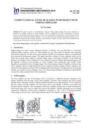
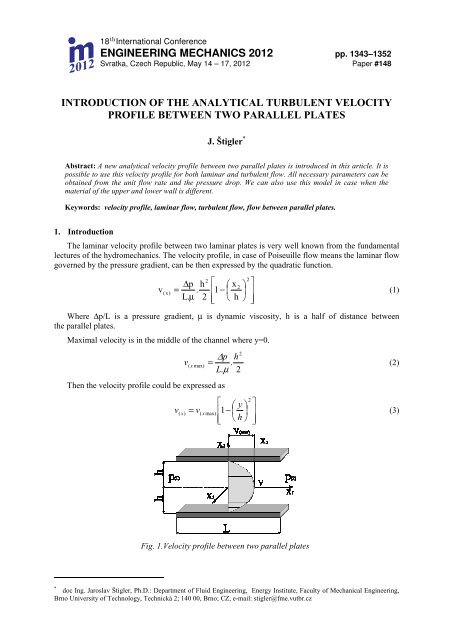
The laminar <strong>velocity</strong> pr<strong>of</strong>ile <strong>between</strong> <strong>two</strong> laminar plates is very well known from <strong>the</strong> fundamental<br />
lectures <strong>of</strong> <strong>the</strong> hydromechanics. The <strong>velocity</strong> pr<strong>of</strong>ile, in case <strong>of</strong> Poiseuille flow means <strong>the</strong> laminar flow<br />
governed by <strong>the</strong> pressure gradient, can be <strong>the</strong>n expressed by <strong>the</strong> quadratic function.<br />
2<br />
2<br />
∆p<br />
h ⎡ ⎛ x ⎤<br />
2 ⎞<br />
v<br />
(x)<br />
= . ⎢1<br />
− ⎜ ⎟ ⎥<br />
(1)<br />
L. µ 2 ⎢⎣<br />
⎝ h ⎠ ⎥⎦<br />
Where ∆p/L is a pressure gradient, µ is dynamic viscosity, h is a half <strong>of</strong> distance <strong>between</strong><br />
<strong>the</strong> parallel plates.<br />
Maximal <strong>velocity</strong> is in <strong>the</strong> middle <strong>of</strong> <strong>the</strong> channel where y=0.<br />
Then <strong>the</strong> <strong>velocity</strong> pr<strong>of</strong>ile could be expressed as<br />
2<br />
∆p<br />
h<br />
v(<br />
x max)<br />
= .<br />
(2)<br />
L.<br />
µ 2<br />
2<br />
⎡ ⎛ y ⎞ ⎤<br />
v( x )<br />
= v(<br />
x max) ⎢1<br />
− ⎜ ⎟ ⎥<br />
(3)<br />
⎢⎣<br />
⎝ h ⎠ ⎥⎦<br />
Fig. 1.Velocity pr<strong>of</strong>ile <strong>between</strong> <strong>two</strong> parallel plates<br />
*<br />
doc Ing. Jaroslav Štigler, Ph.D.: Department <strong>of</strong> Fluid Engineering, Energy Institute, Faculty <strong>of</strong> Mechanical Engineering,<br />
Brno University <strong>of</strong> Technology, Technická 2; 140 00, Brno; CZ, e-mail: stigler@fme.vutbr.cz
1344 Engineering Mechanics 2012, #148<br />
It is more complicated to find any <strong>analytical</strong> solution in <strong>the</strong> case <strong>of</strong> <strong>turbulent</strong> flow. There is some<br />
expression which was found on <strong>the</strong> basis <strong>of</strong> experimental data. It is known as <strong>the</strong> power law.<br />
Unfortunately it was derived only for <strong>the</strong> flow in a pipe with radius R.<br />
v<br />
(x)<br />
n 0<br />
2<br />
⎡ ⎛ r ⎞ ⎤<br />
= v(x max) ⎢1<br />
− ⎜ ⎟ ⎥<br />
(4)<br />
⎢⎣<br />
⎝ R ⎠ ⎥⎦<br />
Where r is a radius within interval , R is <strong>the</strong> pipe radius, n 0 is <strong>the</strong> exponent which is a<br />
function <strong>of</strong> <strong>the</strong> Reynolds number. This exponent can be evaluated from <strong>the</strong> expression<br />
1 Re<br />
= 1+<br />
6<br />
n0 50<br />
There is some discrepancy in this power law definition. It cannot be used near <strong>the</strong> wall, for r=R,<br />
because <strong>the</strong> derivative has an infinite value <strong>the</strong>re. The wall shear stress τ w is <strong>the</strong>n infinite, which does<br />
not correspond with <strong>the</strong> reality.<br />
There is also ano<strong>the</strong>r power law definition by Munson (2006).<br />
(5)<br />
v<br />
(x)<br />
v<br />
(x max)<br />
⎛ r ⎞<br />
⎜1<br />
− ⎟<br />
⎝ R ⎠<br />
1<br />
n 0<br />
= (6)<br />
Where n 0 is a function <strong>of</strong> <strong>the</strong> Reynolds number, see Munson (2006). This <strong>turbulent</strong> <strong>velocity</strong> pr<strong>of</strong>ile<br />
has problems in <strong>two</strong> locations. The first one is <strong>the</strong> same as in <strong>the</strong> previous formulation. The wall shear<br />
stress goes to infinity. The second problematic location is in <strong>the</strong> middle <strong>of</strong> <strong>the</strong> channel, <strong>the</strong> derivative<br />
for r=0 is not zero.<br />
From <strong>the</strong> above examples it is clear that <strong>the</strong>se models have problems near <strong>the</strong> wall. Therefore it is<br />
necessary to focus on <strong>the</strong> near wall region – boundary shear layer. The boundary shear layer in <strong>the</strong><br />
case <strong>of</strong> <strong>turbulent</strong> flow can be divided into three regions.<br />
The first region is called viscous sub-layer. This region is close to <strong>the</strong> wall and <strong>the</strong> viscosity plays<br />
a dominant role in this region. The <strong>velocity</strong> pr<strong>of</strong>ile is linear within this region.<br />
The second region is <strong>the</strong> transition area – this is <strong>the</strong> region <strong>of</strong> smooth transition into <strong>the</strong><br />
logarithmic <strong>velocity</strong> pr<strong>of</strong>ile.<br />
The third one is <strong>the</strong> region where <strong>the</strong> <strong>turbulent</strong> viscosity plays a dominant role.<br />
v x)<br />
v<br />
∗<br />
1 v .y<br />
= .log<br />
κ ν<br />
(<br />
+<br />
B<br />
∗<br />
(7)<br />
We can define dimensionless <strong>velocity</strong> v + and dimensionless distance from <strong>the</strong> wall y + .<br />
v<br />
v<br />
+ = v<br />
(x)<br />
∗<br />
(8)<br />
∗<br />
v .<br />
=<br />
ν<br />
y (9)<br />
+ y<br />
Where shear <strong>velocity</strong> v* is expressed by <strong>the</strong> formula<br />
=<br />
τw<br />
ρ<br />
∗<br />
v (10)<br />
Many different authors use different values <strong>of</strong> constants κ and B. For example Janalík (2008) uses<br />
<strong>the</strong> κ=0,174 and B=5,5 or Munson (2006) uses κ=0,4 and B=5 or Pope (2008) uses κ=0,41 and B 5,2.
Štigler J. 1345<br />
2. Derivation <strong>of</strong> a new <strong>velocity</strong> pr<strong>of</strong>ile<br />
The new <strong>velocity</strong> pr<strong>of</strong>ile is derived on <strong>the</strong> basis <strong>of</strong> <strong>the</strong> vorticity distribution over <strong>the</strong> space <strong>between</strong><br />
<strong>two</strong> parallel plates. This <strong>velocity</strong> pr<strong>of</strong>ile can be used for all, laminar, <strong>turbulent</strong> and constant <strong>velocity</strong><br />
pr<strong>of</strong>ile. The derivation <strong>of</strong> this type <strong>of</strong> <strong>velocity</strong> pr<strong>of</strong>ile is based on a Biott-Savart law, <strong>the</strong> derivation <strong>of</strong><br />
it is made in Brdička 2000, applied on a straight vortex filament with circulation Γ.<br />
v<br />
i<br />
Γ 1<br />
= . . εi3k.<br />
( x'<br />
k<br />
−x<br />
k<br />
)<br />
(11)<br />
2<br />
2. π r<br />
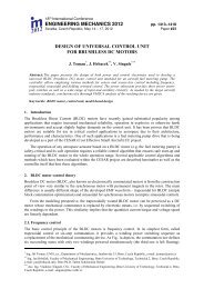
This expression is valid for a special situation when <strong>the</strong> straight vortex filament is parallel to <strong>the</strong> x 3<br />
axis. This is also an expression <strong>of</strong> <strong>the</strong> <strong>velocity</strong> induced by a single potential vortex in case <strong>of</strong> 2D flow<br />
(Lewis 1991). Einstein summation convection is used in <strong>the</strong> expression (11). The v i is <strong>the</strong> <strong>velocity</strong><br />
induced by <strong>the</strong> single vortex, <strong>the</strong> Γ is a circulation around <strong>the</strong> single vortex, x k – are coordinates <strong>of</strong><br />
vortex location, x’ k are coordinates <strong>of</strong> induced <strong>velocity</strong> location, ε ijk is an Levi-Civita tensor <strong>of</strong> 3 rd<br />
order, r is a distance <strong>between</strong> vortex and point <strong>of</strong> induced <strong>velocity</strong>.<br />
Fig. 2.Velocity induced by a single 2D vortex.<br />
Velocity induced by a plain vortex sheet<br />
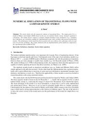
There is ano<strong>the</strong>r well known example <strong>of</strong> <strong>the</strong> <strong>velocity</strong> induced by an infinite plain vortex sheet<br />
Lewis (1991). This sheet consists <strong>of</strong> <strong>the</strong> vortex filaments, with constant circulation Γ which are<br />
parallel to <strong>the</strong> x 3 axis. The situation is depicted in <strong>the</strong> Fig. 3. It is necessary to define linear vorticity<br />
density γ in this case. The circulation dΓ around <strong>the</strong> infinitesimal length <strong>of</strong> sheet ds can be expressed<br />
this way<br />
d Γ = γ .ds =><br />
dΓ<br />
γ = (12)<br />
ds<br />
Fig. 3.Velocity induced by <strong>the</strong> plain vortex sheet<br />
parallel to <strong>the</strong> x 1 ,x 3 plain.<br />
Fig.4. Velocity pr<strong>of</strong>ile induced by a plain<br />
vortex sheet parallel to <strong>the</strong> x 1 ,x 3 plain.
1346 Engineering Mechanics 2012, #148<br />
In case that <strong>the</strong> vorticity density is constant, over <strong>the</strong> whole sheet, <strong>the</strong> <strong>velocity</strong> induced by a vortex<br />
sheet can be expressed this way.<br />
( x'<br />
−x<br />
)<br />
γ<br />
k<br />
vi<br />
= . ε<br />
i3k<br />
.<br />
2 r<br />
Where γ is <strong>the</strong> vorticity density, x’ k are <strong>the</strong> coordinates <strong>of</strong> location where <strong>the</strong> <strong>velocity</strong> is induced,<br />
x (0)k are <strong>the</strong> coordinates <strong>of</strong> x’ k point projection on <strong>the</strong> vortex sheet, r (0) is a distance <strong>of</strong> point x’ k from<br />
<strong>the</strong> vortex sheet. For <strong>the</strong> case depicted in a fig. 3, when <strong>the</strong> vortex sheet is collinear with plane x 1 x 3 ,<br />
<strong>the</strong> <strong>velocity</strong> components are:<br />
γ<br />
v<br />
1<br />
= − ;<br />
2<br />
= 0<br />
2<br />
γ<br />
v<br />
1<br />
= ;<br />
2<br />
= 0<br />
2<br />
(0)<br />
(0) k<br />
v within <strong>the</strong> interval ∈ ( h,<br />
+ ∞)<br />
v within <strong>the</strong> interval ∈ ( h,<br />
− ∞)<br />
' 2<br />
(13)<br />
x (14)<br />
x (15)<br />
This type <strong>of</strong> flow is depicted in <strong>the</strong> fig 4. It means that <strong>velocity</strong> within half-plane above vortex<br />
sheet is constant, parallel to <strong>the</strong> vortex sheet and with <strong>the</strong> orientation to <strong>the</strong> left. Velocity within <strong>the</strong><br />
half-plane below vortex sheet is also parallel to <strong>the</strong> vortex sheet but with <strong>the</strong> orientation to <strong>the</strong> right.<br />
Velocity induced by <strong>two</strong> vortex sheets with <strong>the</strong> opposite vorticity density orientation<br />
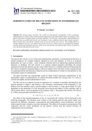
Now it is possible to study fluid flow with <strong>two</strong> parallel vortex sheet s (1) , and s (2) . The magnitude <strong>of</strong><br />
<strong>the</strong> vorticity density <strong>of</strong> both vortex sheets is equal but <strong>the</strong> orientation is opposite. It means that γ (1) =γ<br />
and γ (2) =-γ. The vortex sheet s (1) position is x 2 =h 1 . The vortex sheet s (2) position is x 2 =-h 2 . This<br />
situation is depicted in <strong>the</strong> fig. 5.<br />
' 2<br />
Fig. 5.Velocity induced by <strong>the</strong> <strong>two</strong> plain vortex<br />
sheets parallel to <strong>the</strong> x 1 ,x 3 plain.<br />
Fig.6. Velocity pr<strong>of</strong>ile induced by a plain<br />
vortex sheet parallel to <strong>the</strong> x 1 ,x 3 plain.<br />
The induced <strong>velocity</strong> for this case should be expressed by this formula<br />
i<br />
=<br />
∑<br />
γ<br />
( x' −x<br />
)<br />
n<br />
( j)<br />
k (0 j)k<br />
. εi3k<br />
j = 1 2 r(0 j)<br />
v (16)<br />
This formula is general for an arbitrary number n <strong>of</strong> vortex sheets. It is possible, for case <strong>of</strong> <strong>two</strong><br />
vortex sheets with respect to <strong>the</strong> (16), to write<br />
v<br />
( x'<br />
−x<br />
) ( x'<br />
−x<br />
)<br />
γ<br />
γ<br />
k<br />
2 r<br />
k (01) k<br />
i<br />
= . εi3k<br />
− . εi3k<br />
r(01)<br />
2<br />
(02)<br />
(02) k<br />
Explanation all parameter in above equation are clear from <strong>the</strong> fig. 5.<br />
(17)
Štigler J. 1347<br />
It is possible to have three different solutions now.<br />
v<br />
1<br />
= 0 ;<br />
2<br />
= 0<br />
v = γ ; 0<br />
1<br />
v within <strong>the</strong> interval ∈ ( h,<br />
+ ∞)<br />
v within <strong>the</strong> interval x'<br />
2<br />
( − h, + h)<br />
2<br />
=<br />
v 1<br />
= 0 ; 0<br />
v 2<br />
= within <strong>the</strong> interval ' ( − ∞,<br />
− h)<br />
x (18)<br />
' 2<br />
x 2<br />
∈ (19)<br />
∈ (20)<br />
This solution is very nice and reasonable. It is kind <strong>of</strong> <strong>the</strong> fluid flow <strong>between</strong> <strong>two</strong> parallel plates<br />
for infinite Reynolds number Re=∞.<br />
Now it is only a small step to find <strong>the</strong> expression <strong>of</strong> <strong>the</strong> <strong>velocity</strong> pr<strong>of</strong>ile for <strong>the</strong> finite Reynolds<br />
number.<br />
Velocity pr<strong>of</strong>ile for <strong>the</strong> continuous vorticity distribution over <strong>the</strong> cross-section<br />
It has to be assumed, for this case, that <strong>the</strong> vorticity density is not <strong>the</strong> linear density but it is <strong>the</strong><br />
planar vorticity density. It will be function <strong>of</strong> <strong>the</strong> x 2 coordinate <strong>between</strong> <strong>the</strong> plates. Vorticity density<br />
for <strong>the</strong> fixed coordinate x 2 is constant. The situation is depicted in a fig 7. It is necessary to define <strong>the</strong><br />
coordinate system. The axis x 1 is parallel to <strong>the</strong> plates and it is located in <strong>the</strong> maximal <strong>velocity</strong><br />
position.<br />
Fig. 7.The distribution <strong>of</strong> <strong>the</strong> planar vorticity density <strong>between</strong> <strong>two</strong> plates<br />
The <strong>velocity</strong> pr<strong>of</strong>ile is derived under <strong>the</strong>se assumptions:<br />
• It is <strong>the</strong> fluid flow <strong>between</strong> <strong>two</strong> parallel infinite plane plates.<br />
• The vorticity density distribution is continuous <strong>between</strong> plates. It will be described by <strong>two</strong><br />
polynomial functions γ (1) and γ (2) <strong>of</strong> <strong>the</strong> N th order.<br />
• The unit flow rate Q and <strong>the</strong> pressure drop ∆p are known parameters.<br />
The continuous vorticity density distribution can be expressed by <strong>the</strong> next formulas.<br />
Now <strong>the</strong> <strong>velocity</strong> can be expressed this way<br />
v<br />
1<br />
N<br />
( 1)<br />
= ∑ ( ).<br />
n=<br />
0<br />
n<br />
2<br />
γ A n<br />
x<br />
(21)<br />
N<br />
( 2)<br />
= −∑<br />
( ).<br />
n=<br />
0<br />
n<br />
2<br />
γ B n<br />
x<br />
(22)<br />
n+<br />
1<br />
n+<br />
1<br />
n+<br />
1<br />
( B(<br />
n)<br />
. h2<br />
+ A(<br />
n)<br />
. h1<br />
2. A(<br />
n)<br />
x2<br />
)<br />
N<br />
( + )1<br />
= ∑<br />
− .<br />
n=<br />
0 2.( n + 1)<br />
n+<br />
1<br />
n+<br />
1<br />
n+<br />
1<br />
( B(n)<br />
.h<br />
2<br />
+ A(n)<br />
.h1<br />
− 2.B(n)<br />
.<br />
2<br />
)<br />
N<br />
( −)1<br />
= ∑<br />
x<br />
n=<br />
0 2.(n + 1)<br />
x = 0 h (23)<br />
within <strong>the</strong> interval<br />
1<br />
2<br />
,<br />
1<br />
v within <strong>the</strong> interval x2 − h 2<br />
, 0<br />
= (24)
1348 Engineering Mechanics 2012, #148<br />
It is necessary to determine <strong>the</strong> coefficients A (n) and B (n) for n=1-N. These coefficients can be<br />
determined on <strong>the</strong> basis <strong>of</strong> <strong>the</strong> following conditions.<br />
• Slip condition on <strong>the</strong> walls<br />
v ( + )<br />
= 0 , for x<br />
2<br />
= h1<br />
v ( − )<br />
= 0 , for x2 = −h2<br />
• The unit flow rate is known.<br />
• Circulation around element dx 1 .(h (1) +h (2) ) is zero.<br />
• The necessary number <strong>of</strong> derivative at point x 2 = 0 is zero.<br />
On <strong>the</strong> basis <strong>of</strong> <strong>the</strong>se conditions it is possible to express <strong>velocity</strong> pr<strong>of</strong>ile<br />
(N + 2)<br />
= .<br />
(N + 1) (h<br />
Q<br />
+ h<br />
⎡ ⎛ x<br />
. ⎢1<br />
−<br />
⎜<br />
) ⎢⎣<br />
⎝ h<br />
⎞<br />
⎟<br />
⎠<br />
N + 1<br />
2<br />
v<br />
( + )1<br />
within <strong>the</strong> interval<br />
2<br />
0,<br />
h1<br />
1 2<br />
1<br />
⎤<br />
⎥<br />
⎥⎦<br />
x = (25)<br />
N + 1<br />
(N + 2) Q ⎡ ⎛ x ⎞ ⎤<br />
2<br />
v =<br />
⎢ −<br />
⎜<br />
⎟<br />
( −)1<br />
. . 1 ⎥ within <strong>the</strong> interval x2 − h 2<br />
, 0<br />
(N + 1) (h1<br />
+ h2)<br />
⎢⎣<br />
⎝ h2<br />
⎠ ⎥⎦<br />
The maximal and average <strong>velocity</strong> can be expressed this way<br />
v<br />
v<br />
(max)1<br />
(av)1<br />
(N + 2) Q<br />
.<br />
(N + 1) (h + h )<br />
1<br />
2<br />
= (26)<br />
= (27)<br />
Q<br />
(h + h )<br />
= (28)<br />
1<br />
2<br />
The expression for <strong>the</strong> number N has to be found now. It is possible to do this from <strong>the</strong> known<br />
pressure drop.<br />
h .h<br />
µ .v<br />
(p1<br />
− p )<br />
.<br />
L<br />
= (29)<br />
2<br />
2<br />
N<br />
1<br />
−<br />
(av)<br />
Where µ is <strong>the</strong> dynamic viscosity. All above expressions are derived for a case that <strong>the</strong> plate 1 and<br />
plate 2 were made from different materials. So it means that <strong>the</strong>re could be different conditions on <strong>the</strong><br />
walls. If <strong>the</strong> conditions on <strong>the</strong> plates are identical <strong>the</strong>n <strong>the</strong> <strong>velocity</strong> pr<strong>of</strong>ile will be symmetrical (h 1 =h 2<br />
= h) and it is possible to write<br />
N+1<br />
(N + 2) Q<br />
⎡ ⎛ x ⎤<br />
2<br />
⎞<br />
v ⎢ − ⎜ ⎟ ⎥<br />
1<br />
= . . 1<br />
within <strong>the</strong> interval<br />
(N + 1) 2.h ⎢<br />
x 2<br />
− h, h<br />
⎣ ⎝ h ⎠ ⎥<br />
⎦<br />
h<br />
µ .v<br />
(p<br />
.<br />
− p<br />
L<br />
2<br />
1 2<br />
N<br />
(av)<br />
2<br />
)<br />
− 2<br />
= (30)<br />
= (31)<br />
This expression can be used for all types <strong>velocity</strong> pr<strong>of</strong>iles from laminar <strong>velocity</strong> pr<strong>of</strong>ile (N=1), for<br />
<strong>turbulent</strong> <strong>velocity</strong> pr<strong>of</strong>iles and also for a piston <strong>velocity</strong> pr<strong>of</strong>iles N→∞. There is no problem with <strong>the</strong><br />
derivatives near <strong>the</strong> wall and with <strong>the</strong> zero value <strong>of</strong> <strong>the</strong> first derivative in <strong>the</strong> centre <strong>of</strong> channel.<br />
3. Discussion<br />
The formal comparison <strong>of</strong> different <strong>velocity</strong> pr<strong>of</strong>iles will be presented in this chapter. The only<br />
problem <strong>of</strong> it is that <strong>the</strong> power law <strong>velocity</strong> pr<strong>of</strong>iles are derived for a <strong>turbulent</strong> flow in pipes. But it is
Štigler J. 1349<br />
possible to compare <strong>the</strong> <strong>velocity</strong> pr<strong>of</strong>iles normalized by v max <strong>velocity</strong>. Comparison <strong>of</strong> <strong>velocity</strong> pr<strong>of</strong>iles<br />
is in <strong>the</strong> fig. 8. It is only formal comparison because <strong>the</strong> pressure drop or <strong>the</strong> friction factor for <strong>the</strong><br />
fluid flow <strong>between</strong> <strong>the</strong> parallel plates is not known. Therefore <strong>the</strong> three new <strong>velocity</strong> pr<strong>of</strong>iles for<br />
different values <strong>of</strong> power N are compared with Munson (2006) power law <strong>velocity</strong> pr<strong>of</strong>ile and with<br />
Janalík (2008) power law <strong>velocity</strong> pr<strong>of</strong>ile in <strong>the</strong> fig 8. It is apparent that <strong>the</strong> character all kind <strong>of</strong><br />
<strong>velocity</strong> pr<strong>of</strong>iles are different. The Janalik’s <strong>velocity</strong> pr<strong>of</strong>ile is ra<strong>the</strong>r rounded even for very high<br />
Reynolds number. The Munson <strong>velocity</strong> pr<strong>of</strong>ile has no continuous first derivative in <strong>the</strong> center <strong>of</strong><br />
channel. The new <strong>velocity</strong> pr<strong>of</strong>iles have also a problem that <strong>the</strong>re is a zero second derivative in <strong>the</strong><br />
centre <strong>of</strong> channel. It means that <strong>the</strong>re is an infinite radius <strong>the</strong>re. But this problem should be solved<br />
during derivation its derivation. It means that <strong>the</strong> <strong>velocity</strong> pr<strong>of</strong>ile can be modified in way to ensure non<br />
zero second derivative. But it has not been done yet.<br />
Fig. 8.New <strong>velocity</strong> pr<strong>of</strong>iles in comparison with power law <strong>velocity</strong> pr<strong>of</strong>iles.<br />
It is possible also compare <strong>the</strong> <strong>velocity</strong> pr<strong>of</strong>ile near <strong>the</strong> wall with a logarithm wall law. This<br />
comparison is depicted in a fig. 9.<br />
Fig. 9.The new <strong>velocity</strong> pr<strong>of</strong>iles comparison with log wall law.
1350 Engineering Mechanics 2012, #148<br />
The comparison is not so good because <strong>the</strong> exponent N is not evaluated, because <strong>the</strong>re is no<br />
a measuring <strong>of</strong> pressure drop and flow rate. Therefore <strong>the</strong>re are depicted several <strong>velocity</strong> pr<strong>of</strong>iles for<br />
different exponent N. It is apparent that <strong>the</strong> boundary shear layer in case <strong>of</strong> <strong>the</strong> new <strong>velocity</strong> pr<strong>of</strong>ile is<br />
thinner than in <strong>the</strong> case <strong>of</strong> real <strong>velocity</strong> pr<strong>of</strong>ile. This is probably consequence <strong>of</strong> <strong>the</strong> zero value <strong>of</strong> <strong>the</strong><br />
second derivative <strong>of</strong> <strong>the</strong> <strong>velocity</strong> pr<strong>of</strong>ile in <strong>the</strong> channel centre. There is no comparison for <strong>the</strong> power<br />
law pr<strong>of</strong>iles because <strong>the</strong>re is no possible to express y + and v + because infinite shear stress at <strong>the</strong> wall.<br />
At <strong>the</strong> end it would be interesting to draw <strong>the</strong> shear stress over channel. It is known that <strong>the</strong> total<br />
shear stress is linear. Total shear stress is a sum <strong>of</strong> <strong>the</strong> viscous shear stress τ µ and <strong>the</strong> <strong>turbulent</strong> or<br />
(Reynolds) shear stress τ t .<br />
τ = τµ + τ t<br />
(32)<br />
Viscous shear stress should be expressed from a <strong>velocity</strong> pr<strong>of</strong>ile formula (29).<br />
( N + 1)<br />
⎛ x<br />
⎜<br />
⎝ h<br />
N<br />
2<br />
τ µ<br />
= µ .v(max)<br />
. . within <strong>the</strong> interval x 2<br />
− h, 0<br />
h<br />
( N + 1)<br />
⎞<br />
⎟<br />
⎠<br />
⎛ x<br />
⎜<br />
⎝ h<br />
N<br />
2<br />
τ µ<br />
= −µ .v(max)<br />
. . within <strong>the</strong> interval 0, h<br />
This stress can be expressed in a dimensionless form<br />
h<br />
( N + 1 ).<br />
⎞<br />
⎟<br />
⎠<br />
N<br />
τ µ<br />
.h ⎛ x<br />
2<br />
⎞<br />
= ⎜ ⎟ within <strong>the</strong> interval x 2<br />
− h, 0<br />
µ .v<br />
(max)<br />
⎜<br />
⎝<br />
( N + 1 ).<br />
h<br />
⎟<br />
⎠<br />
N<br />
τ µ<br />
.h<br />
⎛ x<br />
2<br />
⎞<br />
= − ⎜ ⎟ within <strong>the</strong> interval 0, h<br />
µ .v<br />
(max)<br />
⎜<br />
⎝<br />
h<br />
⎟<br />
⎠<br />
= (33)<br />
x 2<br />
= (34)<br />
= (35)<br />
x 2<br />
= (36)<br />
The viscous stress toge<strong>the</strong>r with <strong>the</strong> Reynolds stress for three different exponents N are depicted in<br />
<strong>the</strong> fig. 10. This also can’t be compared with <strong>the</strong> power law <strong>velocity</strong> pr<strong>of</strong>iles because its shear stress at<br />
<strong>the</strong> wall is infinite.<br />
Fig. 10.The Reynolds and viscous stresses derived from a new <strong>velocity</strong> pr<strong>of</strong>ile..
Štigler J. 1351<br />
4. Conclusion<br />
The new <strong>velocity</strong> pr<strong>of</strong>ile based on a vorticity distribution <strong>between</strong> <strong>two</strong> parallel plates has been<br />
presented in this paper. This <strong>velocity</strong> pr<strong>of</strong>ile is better than <strong>the</strong> power law <strong>velocity</strong> pr<strong>of</strong>iles because it<br />
has not infinite shear stress at <strong>the</strong> wall. It means that it is possible to express <strong>the</strong> Reynolds stresses and<br />
it is possible to compare this pr<strong>of</strong>ile with <strong>the</strong> logarithmic law near <strong>the</strong> wall. This is not possible in case<br />
<strong>of</strong> <strong>the</strong> power law <strong>velocity</strong> pr<strong>of</strong>iles because <strong>the</strong>y have infinite derivative near <strong>the</strong> wall. The new<br />
<strong>velocity</strong> pr<strong>of</strong>ile has only one problem which can be removed. The problem is that this pr<strong>of</strong>ile has zero<br />
second derivative in <strong>the</strong> centre <strong>of</strong> channel. It means that <strong>the</strong>re is an infinite radius <strong>of</strong> curvature. It is<br />
also necessary to compare this <strong>velocity</strong> pr<strong>of</strong>ile directly with an experimental <strong>velocity</strong> pr<strong>of</strong>iles. This<br />
work can help in understanding or even in modeling <strong>of</strong> boundary shear layers in CFD s<strong>of</strong>tware.<br />
List <strong>of</strong> Symbols<br />
Symbol Units Description<br />
A (n) Varies Polynom coefficients<br />
B (n) Varies Polynom coefficients<br />
h [m] Half distance <strong>between</strong> <strong>two</strong> parallel plates<br />
h 1 , h 2 [m] Distance <strong>of</strong> plate s 1 /s 2 from a coordinate system origin<br />
L [m] Length. Distance <strong>between</strong> <strong>the</strong> pressure location measuring.<br />
n 0 - Exponent<br />
∆p [Pa] Pressure difference<br />
p (1) , p (2) [Pa] Pressure at location 1 or 2 respectively<br />
Q [m] Unit flow rate. Flow rate <strong>between</strong> <strong>two</strong> parallel plates with 1m width.<br />
r, R [m] Radius<br />
Re [-] Reynolds number<br />
r (0) [m] Distance <strong>of</strong> point x’ k from vortex sheet<br />
v (av) [m.s -1 ] Average <strong>velocity</strong> <strong>between</strong> <strong>two</strong> parallel plates<br />
v (x) [m.s -1 ] Component <strong>of</strong> <strong>velocity</strong> in x direction<br />
v (x max) [m.s -1 ] Maximal <strong>velocity</strong> component in x direction<br />
v* [m.s -1 ] Shear <strong>velocity</strong><br />
v + [-] Dimensionless <strong>velocity</strong> near <strong>the</strong> wall<br />
v i [m.s -1 ] Velocity vector<br />
v 2 , v 2 , v 3 [m.s -1 ] Components <strong>of</strong> <strong>velocity</strong> vector<br />
x 1 , x 2 , x 3 [m] Coordinates <strong>of</strong> location<br />
x' k [m] Coordinates <strong>of</strong> <strong>the</strong> induced <strong>velocity</strong> point<br />
x (0)k [m] Coordinates <strong>of</strong> point x’ k projected onto <strong>the</strong> vortex sheet<br />
y [m] Coordinate y, or distance from wall<br />
y + [-] Dimensionless distance from <strong>the</strong> wall<br />
Γ [m 2 .s -1 ] Circulation<br />
γ [m.s -1 ]/ [s -1 ] Linear /planar vorticity density<br />
µ [Pa.s] Dynamic viscosity<br />
ν [m 2 .s -1 ] Kinematic viscosity<br />
ε ijk [-] Levi-Civita tensor<br />
τ µ [Pa] Viscous shear stress<br />
τ t [Pa] Turbulent (Reynolds) shear stress
1352 Engineering Mechanics 2012, #148<br />
Acknowledgement<br />
This research was funded by Brno University <strong>of</strong> Technology, Faculty <strong>of</strong> Mechanical Engineering<br />
through project with number FSI-S-12-2.<br />
References<br />
Pope, S.B. (2008) Turbulent Flows. Fifth printing, Cambridge University Press, ISBN 978-0-521-59889-6.<br />
Janalík, J. (2008) Vybrané kapitoly z mechaniky tekutin. VŠB – Technická univerzita Ostrava, ISBN 978-80-<br />
248-1910-5<br />
Munson, B.R. & Young, D. F. & Okiishi, T.H. (2006) Fundamentals <strong>of</strong> Fluid Mechanics, Fifth Edition, John<br />
Wiley & Sons, Inc., ISBN 978-0-471-67582-2.<br />
Brdička, M. & Samek, L. & Sopko, B. (2000) Mechanika kontinua. Akademie věd České republiky,<br />
ACADEMIA, ISBN 80-200-0772-5.<br />
Lewis, R.I. (1991) Vortex Element Mehods for Fluid Dynamics Analysis <strong>of</strong> Engineering Systems. Cambridge<br />
Engine Technology Series, Cambridge University Press, ISBN 0-521-36010-2.