Open source FEM-DEM coupling - Engineering Mechanics

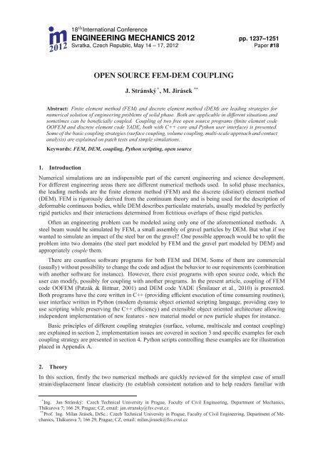
. 18m 2012th International ConferenceENGINEERING MECHANICS 2012 pp. 1237–1251Svratka, Czech Republic, May 14 – 17, 2012 Paper #18OPEN SOURCE FEM-DEM COUPLINGJ. Stránský * ,M.Jirásek **Abstract: Finite element method (FEM) and discrete element method (DEM) are leading strategies fornumerical solution of engineering problems of solid phase. Both are applicable in different situations andsometimes can be beneficially coupled. Coupling of two free open source programs (finite element codeOOFEM and discrete element code YADE, both with C++ core and Python user interface) is presented.Some of the basic coupling strategies (surface coupling, volume coupling, multi-scale approach and contactanalysis) are explained on patch tests and simple simulations.Keywords: FEM, DEM, coupling, Python scripting, open source1. IntroductionNumerical simulations are an indispensible part of the current engineering and science development.For different engineering areas there are different numerical methods used. In solid phase mechanics,the leading methods are the finite element method (FEM) and the discrete (distinct) element method(DEM). FEM is rigorously derived from the continuum theory and is being used for the description ofdeformable continuous bodies, while DEM describes particulate materials, usually modeled by perfectlyrigid particles and their interactions determined from fictitious overlaps of these rigid particles.Often an engineering problem can be modeled using only one of the aforementioned methods. Asteel beam would be simulated by FEM, a small assembly of gravel particles by DEM. But what if wewanted to simulate an impact of the steel bar on the gravel? One possible approach would be to split theproblem into two domains (the steel part modeled by FEM and the gravel part modeled by DEM) andappropriately couple them.There are countless software programs for both FEM and DEM. Some of them are commercial(usually) without possibility to change the code and adjust the behavior to our requirements (combinationwith another software for instance). However, there exist programs with open source code, which theuser can modify, possibly for coupling with another programs. In the present article, coupling of FEMcode OOFEM (Patzák & Bittnar, 2001) and DEM code YADE (Šmilauer et al., 2010) is presented.Both programs have the core written in C++ (providing efficient execution of time consuming routines),user interface written in Python (modern dynamic object oriented scripting language, providing easy touse scripting while preserving the C++ efficiency) and extensible object oriented architecture allowingindependent implementation of new features - new material model or new particle shapes for instance.Basic principles of different coupling strategies (surface, volume, multiscale and contact coupling)are explained in section 2, implementation issues are covered in section 3 and specific examples for eachcoupling strategy are presented in section 4. Python scripts controlling these examples are for illustrationplaced in Appendix A.2. TheoryIn this section, firstly the two numerical methods are quickly reviewed for the simplest case of smallstrain/displacement linear elasticity (to establish consistent notation and to help readers familiar with* Ing. Jan Stránský: Czech Technical University in Prague, Faculty of Civil Engineering, Department of Mechanics,Thákurova 7; 166 29, Prague; CZ, email: jan.stransky@fsv.cvut.cz** Prof. Ing. Milan Jirásek, DrSc.: Czech Technical University in Prague, Faculty of Civil Engineering, Department of Mechanics,Thákurova 7; 166 29, Prague; CZ, email: milan.jirasek@fsv.cvut.cz

1238 Engineering Mechanics 2012, #18one method to understand the other one). Then the basic principles of the chosen coupling strategies areexplained.2.1. Finite element methoddiscretizationFig. 1: Simplified illustration of FEM discretizationThe continuous (static) linear elasticity solves the boundary value problemε = ∇ sym u x ∈ Ω (1)σ = 4 D : ε x ∈ Ω (2)∇ · σ + b = 0 x ∈ Ω (3)u = u x ∈ Γ u (4)n · σ = t x ∈ Γ t (5)where x = vector of Cartesian coordinates, u = u(x) = displacement vector, ε = ε(x) = strain tensor,σ = σ(x) = stress tensor, 4 D = 4 D(x) = fourth-order stiffness tensor, b = b(x) = body forces,t=t(x) = surface tractions, Ω = domain of the problem, Γ u = boundary of the domain with prescribeddisplacements, Γ t = boundary of the domain with prescribed tractions and n = n(x) = outer unitnormal vector of the boundary. ∇ is the vector of spatial partial derivatives, · is contraction and : isdouble contraction (tensor operations). Overbars indicate prescribed values.Combining geometric equations (1), constitutive equations (2) and equilibrium (Cauchy) equations(3) yields Lamé equations∇ · [4 D : (∇u) ] + b = 0, (6)which describe the elasticity problem in the strong sense.The basic idea of FEM is to discretize the domain Ω into finite elements. On each element e, thedisplacement field u e (x) is approximated as a combination of nodal displacement values {d} e . Fromthe element geometry and material parameters, the element stiffness matrix [K] e can be constructed,providing the relationship between the nodal displacements {d} e and nodal internal forces {f} e (7).Approximating the load by nodal forces, the global system of equations[K] e {d} e = {f} e → [K] g {d} g = {f} g (7)is assembled and unknown nodal displacements are solved for defined boundary conditions. Equation(7) can be derived from the virtual work principle and describes the elasticity problem in the weak sense.2.2. Discrete element methodConsider an assembly of rigid particles. The contact (bond, interaction etc.) c between particles iscreated either initially in the beginning of the simulation or when the particles overlap. The contact (seeequations (8-9) and figure 2) can be described by a branch vector l c (connecting the centers of linkedparticles) with normal n c = l c /|l c | . The (linearized) relative contact displacement u c can be expressedin terms of particle displacement x p and rotation ϕ p and decomposed into the normal component u c Nand the shear component u c T. Constitutive (linear elastic) contact law is also expressed (independently)in the normal and shear directions in terms of the normal and shear forces fN c and f T c and normal andshear contact stiffnesses kN c and kc T . The total contact force f c is composed from normal and shear

Stránský J., Jirásek M. 1239u c N nc u c f c f c N ncf c N ncf c Tu c Tn cl cf c TFig. 2: Simplified illustration of the contact displacement and contact forces and their decompositionscomponents. The contact force is considered to act at the contact point (in the middle between particlecenters for example), and so its shear component also causes a moment on both particles.u c N = uc · n c , u c = u c N nc + u c T (8)f c N = k c Nu c N , f c T = k c T u c T , f c = f c Nn c + f c T (9)For each particle p, the forces are then summed from all particles contacts and the Newton’s equationsof motionf p = ∑ f c , ü p = f pm p (10)c∈pare solved using Verlet explicit time integration scheme. m p is the mass of particle p and ü p its acceleration.The summation and integration of the equation of motion is also defined for moments and angularaccelerations. For more details about time integration as well as DEM in general see (Šmilauer et al.,2010) or (Kuhl et. al, 2001).2.3. Surface couplingẋ pẋ pf e FEMf p DEM ∝ ẍpcontact1) 2) 3)Fig. 3: Illustration of FEM/DEM surface couplingThe so-called surface coupling (Fakhimi, 2009; Nakashima & Oida, 2004; Oñate & Rojek, 2004;Villard et al., 2009) is probably the most straightforward coupling method. The principle is to split thewhole problem into two non-overlapping domains, one modeled by FEM and the other by DEM (asalready illustrated on the steel beam – gravel example in the introduction). As long as there is no overlapbetween the two domains, nothing special happens - both methods are applied independently.If a contact between a finite element and a DEM particle is detected, the new force becomes acting onthe DEM particle (causing its acceleration). The same force (with the same magnitude and the oppositedirection) of course acts also on the FEM element and is processed as a load boundary condition, seefigure 3.

1240 Engineering Mechanics 2012, #18In the current OOFEM/YADE implementation, the FEM boundary (surface) elements are copiedinto DEM part as special particles. This approach allows us to exploit efficient YADE contact detectionalgorithms. The resulting DEM force and moment acting on surface element are in FEM part transferedinto nodal forces and further assumed as external load.2.4. Volume couplingFEM contributiontrans. zoneDEM contribution(a)(b)Fig. 4: Illustration of ”master/slave” (a) and ”Arlequin” (b) FEM/DEM volume couplingVolume coupling is similar to the surface coupling. The difference is that the two subdomains overlapeach other. The possible usage of this approach could be a model of concrete beam subjected to an impactload (blast for example). The whole beam would be modeled by FEM and only a small volume of theconcrete (the volume to be fragmented and crushed) would be modeled by DEM.There are two basic strategies how to model transition between FEM and DEM domains. The firstone, ”direct” or ”master/slave” method, (Azvedo & Lemos, 2004) considers DEM particles overlappingwith FEM as direct slaves of the FEM mesh (using standard ”master/slave” or ”hanging nodes” approach).The second one, the ”Arlequin” method (Rousseau et al., 2009; Wellmann & Wriggers, 2012),considers a transition bridging zone, where the total response is superposed from contributions of thetwo models and is interpolated between both domains.2.5. Multiscale couplingMacro (FEM)stiffnessstressstrainMicro (DEM)solving BVPFig. 5: Illustration of multiscale coupling according to (Geers et. al, 2010) applied to FEM/DEMThe idea of multiscale simulations is to model the problem on the large (macro) scale using informationfrom a lower (micro) scale. In the current context, the (first order) homogenization (Geers et. al,2010) is presented. Geometric information (strain) from macro scale (Gauss points of FEM mesh) istransfered to the micro scale (representative volume element - RVE - modeled by DEM), see figure 5.On the micro scale, the boundary value problem (BVP) governed by the transfered prescribed strain issolved using periodic boundary conditions (Stránský & Jirásek, 2010). The output of the micro-scaleproblem are the stress tensor and the constitutive characteristics (stiffness tensor), which are transferedback to the macro-scale problem.

Stránský J., Jirásek M. 1241As an example of this approach, consider a model of a large sample of sand. On macro scale, sandis usually considered as a continuous material. DEM modeling of a large sand sample with individualgrains modeled by individual particles would not be feasible. According to these two facts, the macroscale problem is modeled by FEM. However, the particular nature of sand is preserved in the microscaleRVE simulations, which provides the FEM part with stress and stiffness. Thus we do not need anyexplicit expression of the material law on the FEM scale (it is determined from the actual micro RVEresponse).The stress and stiffness can be evaluated either analytically or numerically. The analytical formulas(Kuhl et. al, 2001) are inspired by the microplane theory and are derived from Voigt’s hypothesis. Itassumes that the strain ε is distributed uniformly in the RVE and, consequently, the relative displacementu c of each contact c can be expressed and decomposed in the form (see (Kuhl et. al, 2001) and equations(8-9) for more details):u c = ε · l c = |l c | ε · n c = u c Nn c + u c T (11)u c N = uc · n c = (|l c | ε · n c ) · n c = |l c | (n c ⊗ n c ) : ε = |l c | N c : ε (12)u c T = uc −u c N nc = |l c | ε·n c − |l c | ε : (n c ⊗n c )n c = |l c | ε : (I sym·n−n⊗n⊗n) = |l c | T c : ε (13)N c =n c ⊗n c and T c =I sym·n c −n c ⊗n c ⊗n c are auxiliary projection tensors and I sym = 1 2 [δ ilδ jk +δ ik δ jl ]is the fourth order symmetric identity tensor. The equivalence of macroscopic (M) and microscopic (m)virtual workσ : δε = δW M = δW m = 1 ∑f c · δu c = 1 ∑f c · δε · l c = 1 ∑[f c ⊗ l c ] : δε (14)VVVc∈Vyields the expression for the stress tensor (with substitution of equations (8) and (9))c∈Vc∈Vσ = 1 ∑[f c ⊗ l c ] sym = 1 ∑|l c | (N c fN c + [fT c ⊗ n c ] sym ). (15)VVSubstituting equations (9), (12) and (13) into (15)= 1 Vσ = 1 Vc∈V∑|l c | (N c kNu c c N + [n c ⊗ kT c u c T ] sym ) =c∈V∑|l c | (N c kN c |lc | N c : ε + [n c ⊗ kT c |lc | T c : ε] sym ) = (16)c∈V= 1 V∑|l c | 2 (kN c Nc ⊗ N c + kT c [nc ⊗ T c ] sym ) : εc∈Vand comparing (16) with (2) yields the expression for the stiffness tensor4 D = 1 VD ijkl = 1 V∑|l c | 2 (kN c N c ⊗ N c + kT c [n c ⊗ T c ] sym )c∈V∑|l c |[(k 2 N c − kT c )n c in c jn c k nc l + 1 ( kc T nc4 i n c l δ jk + n c in c k δ jl + n c jn c l δ ik + n c jn c k δ ) ]il .c∈VThis estimation of the stiffness tensor is derived from the kinematic constraint, thus it is an upperbound of the real one. If the real strain state differs too much from the assumed uniform state (strainlocalization for instance), the analytical stiffness estimation is no more valid and the stiffness has to becomputed numerically. The aspect of strain localization can be in same cases captured by the implementedperiodic boundary conditions, see (Šmilauer et al., 2010) and (Stránský & Jirásek, 2010), but itwill be among other aspects (second order homogenization for instance) subjected to further analysis anddevelopment.c∈V(17)

1242 Engineering Mechanics 2012, #182.6. Contact analysisThe idea of contact analysis (Frenning, 2009) is very simple and opposite to the multiscale approach.The material on the large scale is considered to be of a particulate nature and is modeled by particlesusing DEM. Each such particle is further modeled by FEM.There is no strict border between the cases when the solution can be considered as contact FEManalysis and when it is already DEM. For only a few particles we would probably use the former one, butwhen the number of particles is large, the DEM modeling (with its efficient contact detection algorithms)would be more convenient. This strategy can be actually considered as full FEM, only the contactdetection is ”borrowed” from the DEM program.DEMFEMFig. 6: Illustration of multimethod FEM/DEM contact analysis3. ImplementationThe current implementation serves only for testing of the methods and functionality, therefore not allfeatures are in public versions of OOFEM and YADE yet. Since this paper is about open source coupling,the changes will be (after further testing and bug-fixing) of course merged to public versions and will beavailable for any potential user/developer.From the point of view of Python, all important functionality is concentrated into the fakemupifmodule, which provides several classes derived from the base FemDemCoupler class. Each suchclass has its step method, which is the only needed additional command in comparison with noncoupledsimulations (see the example scripts in the following sections). When the testing is finished,the functionality (probably with some syntax and internal code modifications, but with same high-levelsimplicity) will be implemented into the MuPIF project (Patzák, 2011) to enable coupling with otherprograms or other physical models (heat transfer for instance).Python(module fakemupif)MuPIFOOFEMPythoninterfaceOOFEMYADEPythoninterfaceYADE(a)OOFEMOOFEM APIOOFEMPythoninterface(b)YADE APIYADEPythoninterfaceYADEFig. 7: Current (testing) (a) and planned (b) implementation4. ExamplesIn this section, one specific simple example for each discussed coupling strategy is presented.

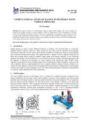
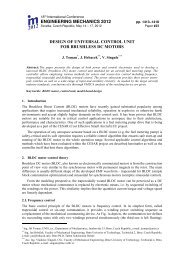
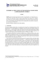
Stránský J., Jirásek M. 1243(a) (b) (c)Fig. 8: Results of surface coupling - soil-tire contact:simulation setup (a), detail of contact (b) and resulting vertical normal stress in FEM domain (c)4.1. Surface coupling: soil-tire contactSimulation of the soil-tire contact, inspired by (Nakashima & Oida, 2004), is presented here. The tireis modeled by FEM as a linear elastic material, the soil is modeled by DEM as spherical particles. Ofcourse, in a real simulation we could use a more complicated soil grain geometry, a more advanced (thanjust linear elastic) material model for the tire and so on, but for an illustrating and testing example thepresent assumptions are sufficient. See figure 8 and codes 1 and 5.4.2. Volume coupling: three point bendingFig. 9: Results of three point bending:initial state (a), undeformed and deformed final state (b) and normal stress (c)In this example, a simply supported beam was simulated. The whole beam body was simulated byFEM, only the part with maximal tensile normal stress was simulated by DEM. The vertical displacementof the middle cross section was prescribed.Again, the elastic solution is nothing special here, but instead of linear elastic particles we coulduse a kind of material model for fracture description (Azvedo & Lemos, 2004), thus the expected crackinitiation and propagation in the middle cross section would be modeled with the help of discrete models.See figure 9 and codes 2 and 6.4.3. Multiscale coupling: uniaxial strainUniaxial strain (oedometric test) of a sample consisting of two different (linear elastic) materials (withstiffness ratio 1/2) is simulated in this example. The macro-scale problem is modeled by two brickelements. Each FEM element has eight integration points. For each integration point, a DEM microscaleRVE simulation is performed, in which the FEM prescribed strain is imposed. The resulting stressand stiffness are transfered back to the macro-scale FEM simulation.In figure 10, magnified results are plotted. In each material, one micro RVE result is displayed (allRVEs in the same material, due to the simulation setup, correspond to each other). The results of linearelastic behavior are not extremely spectacular indeed, but using nonlinear behavior of RVEs (resulting

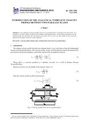
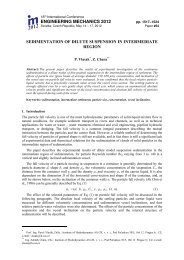
1244 Engineering Mechanics 2012, #18Fig. 10: Results of multiscale uniaxial strain testin higher stiffness when more inter-particle contact occur for instance) could be very useful for certainapplications.See figure 10 and codes 3 and 7.4.4. Contact analysis: cantilever shock analysisIn this example, the simulation of a cantilever shock is presented. The shock is caused by the fall of animpactor – another beam in our example – on the end of the cantilever. Both cantilever and the fallingbeam are modeled by FEM, only a detection algorithm is borrowed from DEM. This contact detectionbetween particles of FEM elements shapes (tetrahedra or bricks) is a typical example of the code, whichis not public yet and needs more testing to be committed to public version. See figure 11 and codes 4and 8.Fig. 11: Results of cantilever shock analysis – different stages of impact5. ConclusionsThe basic principles of the most popular FEM/DEM coupling strategies (surface, volume, multiscale andcontact coupling) were presented, together with specific examples and corresponding Python scripts. Allmethods can be arbitrarily combined with each other or with different methods/programs (which usesPython user interface).As an example, consider a dynamic soil compaction. The compacted soil would be definitely modeledby DEM, the compactor by FEM (here we have surface coupling) and the rest of the soil domainby FEM. The soil DEM / soil FEM interface would probably be of a volume coupling kind. Of course,the FEM soil could be modeled using the multiscale approach, and we could go in coupling further andfurther.

Stránský J., Jirásek M. 1245This example was just to show the variety of possible coupling combinations and that there are a lotof real world problems, where such coupled methods could be useful. Together with the simplicity ofcreating, modifying and running such simulations and extensibility of the used programs (due to the opensource character of the code) it makes this approach attractive for a variety of engineering problems.Future work on this topic will address (among others) second order DEM homogenization, adjustmentof DEM periodic boundary conditions for arbitrary localization analysis, implementation and testingof Arlequin volume coupling method, implementation of contact detection algorithms of FEM elementshaped particles and implementation of testing fakemupif interface into MuPIF framework.AcknowledgmentsFinancial support of the Czech Technical University in Prague under project SGS12/027/OHK1/1T/11 isgratefully acknowledged.ReferencesAzvedo, N. M. & Lemos, L. V. (2006) Hybrid discrete element/finite element method for fracture analysis. ComputerMethods in Applied Mechanics and Engineering, 195, pp. 4579–4593.Fakhimi, A. (2009) A hybrid discretefinite element model for numerical simulation of geomaterials. Computersand Geotechnics, 36, pp. 386–395.Frenning, D. (2008) An efficient finite/discrete element procedure for simulating compression of 3D particle assemblies.Computer Methods in Applied Mechanics and Engineering, 197, pp. 4266–4272.Geers, M. G. D., Kouznetsova, Brekelmans, W. A. M. (2010) Multi-scale computational homogenization: Trendsand challenges. Journal of Computational and Applied Mathematics, 234, pp. 2175–2182.Kuhl, E., DAddetta, G. A., Leukart, M. and Ramm, E. (2001) Microplane modelling and particle modelling ofcohesive-frictional materials. In: Continuous and Discontinuous Modelling of Cohesive-Frictional Materials(P. A. Veemer et al. eds). Springer, Berlin, pp. 31–46Nakashima, H. & Oida, A. (2004) Algorithm and implementation of soiltire contact analysis code based on dynamicFEDE method. Journal of Terramechanics, 41, pp. 127–137.Oñate, E. & Rojek, J. (2004) Combination of discrete element and finite element methods for dynamic analysis ofgeomechanics problems. Computer Methods in Applied Mechanics and Engineering, 193, pp. 3087–3128.Patzák, B. & Bittnar, Z. (2001) Design of object oriented finite element code. Advances in Engineering Software,32, pp. 759–767.Patzák, B. (2011) MuPIF: A Distributed Multi-Physics Integration Tool. In: Proceedings of the Second InternationalConference on Parallel, Distributed, Grid and Cloud Computing for Engineering (P. Ivnyi & B. H. V.Topping eds.). Stirlingshire, United Kingdom, paper 15.Rousseau, J., Frangin, E., Marin, P. & Daudeville, L. (2009) Multidomain finite and discrete elements method forimpact analysis of a concrete structure. Engineering Structures, 31, pp. 2735–2743.Stránský, J. & Jirásek, M. (2010) Calibration of particle-based models using cells with periodic boundary conditions.In: Proc. II International Conference on Particle-based Methods - Fundamentals and Applications (E.Oñate and D.R.J. Owen eds.), CIMNE, Barcelona, pp. 274–285.Šmilauer, V., Catalano, E., Chareyre, B., Dorofeenko, S., Duriez, J., Gladky, A., Kozicki, J., Modenese, C.,Scholtès, L., Sibille, L., Stránský, J. & Thoeni, K. (2010) Yade Documentation (V. Šmilauer ed.),The Yade Project, 1st ed. http://yade-dem.org/doc/.Villard, P., Chevalier, B., Le Hello, B. & Combe, G. (2009) Coupling between finite and discrete element methodsfor the modelling of earth structures reinforced by geosynthetic. Computers and Geotechnics, 36, pp. 709–717.Wellmann, C. & Wriggers, P. (2012) A two-scale model of granular materials. Computer Methods in AppliedMechanics and Engineering, 205–208, pp. 46–58.Xu, M., Gracie, R. & Belytschko, T. (2002) Multiscale Modeling with Extended Bridging Domain Method. In:Bridging the Scales in Science and Engineering (J. Fish ed.). Oxford University Press.

1246 Engineering Mechanics 2012, #18Appendix A.Example scripts and input filesPython scripts controlling examples in section 4 are presented in this section.Currently, OOFEM simulations use input text files, while YADE constructs the simulation directlyin a Python script. Therefore the OOFEM input files (or a significant parts of them) are followed by theactual Python scripts.Since the fakemupif module will be changed and adjusted to MuPIF requirements, the actualcode fakemupif is not presented. However, the simplicity of coupler.step() line (from the userpoint of view representing the entire coupling process) should be preserved.test_surface.oofem.outsurface coupling test - tire-soil contactLinearStatic nsteps 1000 nmodules 1vtk 1 tstep_step 20 domain_all vars 2 1 4 primvars 1 1domain 3dOutputManager tstep_all dofman_all element_allndofman 64 nelem 192 ncrosssect 1 nmat 1 nbc 2 nic 0 nltf 2node 1 coords 3 -3.000000e-01 0.000000e+00 -1.000000e-01 bc 3 0 0 0...node 34 coords 3 0.000000e+00 0.000000e+00 -1.000000e-01 bc 3 1 2 1...node 64 coords 3 -1.307587e-01 1.822355e-01 -4.467372e-02 bc 3 0 0 0ltrspace 1 nodes 4 32 40 42 45 crosssect 1 mat 1...ltrspace 192 nodes 4 38 32 55 46 crosssect 1 mat 1SimpleCS 1 thick 1.0 width 1.0IsoLE 1 d 0. E 100e9 n 0.4 talpha 0.0BoundaryCondition 1 loadTimeFunction 1 prescribedvalue 0.0BoundaryCondition 2 loadTimeFunction 2 prescribedvalue 1.0ConstantFunction 1 f(t) 1.0PiecewiseLinFunction 2 npoints 3 t 3 0 500 1000 f(t) 3 0 0.01 0Code 1: test surface.oofem.intest_volume.oofem.outvolume coupling test - hanging nodes - three point bendingNonLinearStatic nsteps 50 nmodules 1vtk 1 tstep_step 1 domain_all vars 2 1 4 primvars 1 1domain 3dOutputManager tstep_all dofman_all element_allndofman 2478 nelem 1764 ncrosssect 1 nmat 1 nbc 2 nic 0 nltf 1node 1 coords 3 0.000000e+00 0.000000e+00 0.000000e+00 bc 3 0 1 0...node 2478 coords 3 6.000000e+00 3.000000e-01 4.000000e-01 bc 3 0 1 1lspace 1 nodes 8 2 9 58 51 1 8 57 50 crosssect 1 mat 1...lspace 1800 nodes 8 2422 ... 2470 crosssect 1 mat 1SimpleCS 1 thick 1.0 width 1.0IsoLE 1 d 0. E 40e9 n 0.2 talpha 0.0BoundaryCondition 1 loadTimeFunction 1 prescribedvalue 0.0BoundaryCondition 2 loadTimeFunction 1 prescribedvalue 1e-2PiecewiseLinFunction 1 npoints 2 t 2 0 50 f(t) 2 0. 1.Code 2: test volume.oofem.in

Stránský J., Jirásek M. 1249# example script for volume coupling - three point ending# first import required modulesimport fakemupiffrom fakemupif import oofem,yade# then instanciate FEM ...oofemFile = ’test_volume.oofem.in’fem = fakemupif.instanciateOofemProblem(oofemFile)# ... as well as DEM problemdem = yade.Omega()dem.materials.append(fakemupif.defaultMat)rect = yade.pack.inAlignedBox((2.8,0.0,0.12),(3.2,0.3,0.4))sphs = yade.pack.randomDensePack(rect,0.02,spheresInCell=1000)dem.bodies.append(sphs)#coupler = fakemupif.VolumeFemDemCoupler(fem,dem,oofemFile)#dem.dt = .5*yade.utils.SpherePWaveTimeStep(.02,1000,25e9)dem.engines=[yade.ForceResetter(),yade.InsertionSortCollider([yade.Bo1_Sphere_Aabb(aabbEnlargeFactor=1.5,label=’is2aabb’)]),yade.InteractionLoop([yade.Ig2_Sphere_Sphere_Dem3DofGeom(distFactor=1.5,label=’ss2d3dg’)],[yade.Ip2_CpmMat_CpmMat_CpmPhys()],[yade.Law2_Dem3DofGeom_CpmPhys_Cpm()]),yade.NewtonIntegrator(damping=.3),]dem.step()is2aabb.aabbEnlargeFactor = ss2d3dg.distFactor = -1.# Yade vtk exportimport yade.exportvtk = yade.export.VTKExporter(’test_volume.yade’,startSnap=1)# run 50 steps of simulation and save resultsfor i in xrange(50):coupler.step()vtk.exportSpheres(what=[(’dspl’,’b.state.displ()’)])# exitprint ’Finished!’fem.terminateAnalysis()dem.exitNoBacktrace()Code 6: controlling script for three point bending volume coupling example

1250 Engineering Mechanics 2012, #18# example script for multiscale coupling - uniaxial strain# first import required modulesimport fakemupiffrom fakemupif import oofem,yade# then instanciate FEM ...oofemFile = ’test_multi.oofem.in’fem = fakemupif.instanciateOofemProblem(oofemFile)# ... as well as DEM problemdem = yade.Omega()demMat1 = dem.materials.append(fakemupif.defaultMat)demMat2 = dem.materials.append(fakemupif.defaultMat2)#coupler = fakemupif.MultiScaleFemDemCoupler(fem,dem,oofemFile)## Yade vtk exportimport yade.exportvtks = {}for gp in coupler.gps:newScene = dem.addScene()coupler.scenes.append(newScene)dem.switchToScene(newScene)dem.dt = .5*yade.utils.SpherePWaveTimeStep(.001,1000,25e9)dem.bodies.append(yade.pack.randomPeriPack(.001,.02))dem.engines=[yade.ForceResetter(),yade.InsertionSortCollider([yade.Bo1_Sphere_Aabb(aabbEnlargeFactor=1.5,label=’is2aabb’)]),yade.InteractionLoop([yade.Ig2_Sphere_Sphere_Dem3DofGeom(distFactor=1.5,label=’ss2d3dg’)],[yade.Ip2_CpmMat_CpmMat_CpmPhys()],[yade.Law2_Dem3DofGeom_CpmPhys_Cpm()]),yade.NewtonIntegrator(damping=.3),]dem.step()is2aabb.aabbEnlargeFactor = ss2d3dg.distFactor = -1.vtks[newScene] = yade.export.VTKExporter(’test_multi.yade%d’%newScene)# run 50 steps of simulation and save resultsfor i in xrange(50):coupler.step()for scene in coupler.scenes:vtks[scene].exportSpheres(what=[(’dspl’,’b.state.displ()’)])# exitprint ’Finished!’fem.terminateAnalysis()dem.exitNoBacktrace()Code 7: controlling script for multiscale uniaxial strain simulation

Stránský J., Jirásek M. 1251# example script for contact coupling - cantilever impact# first import required modulesimport fakemupiffrom fakemupif import oofem,yadenSteps = 12000# then instanciate FEM ...oofemFile = ’test_contact.oofem.in’fem = fakemupif.instanciateOofemProblem(oofemFile)# ... as well as DEM problemdem = yade.Omega()dem.materials.append(fakemupif.defaultMat)#coupler = fakemupif.ContactFemDemCoupler(fem,dem,oofemFile)#dem.bodies.append(coupler.demImages)dem.engines=[yade.ForceResetter(),yade.InsertionSortCollider([yade.Bo1_Facet_Aabb()]),yade.InteractionLoop([yade.Ig2_Facet_Facet_Dem3DofGeom()],[yade.Ip2_CpmMat_CpmMat_CpmPhys()],[yade.Law2_Dem3DofGeom_CpmPhys_Cpm()]),]# runfor i in xrange(nSteps):coupler.step()# exitprint ’Finished!’fem.terminateAnalysis()dem.exitNoBacktrace()Code 8: controlling script for cantilever shock analysis