non-newtonian effects of pulsatile blood flow in a realistic bypass ...

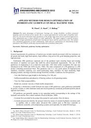
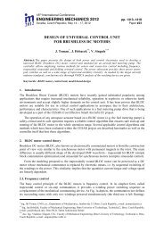
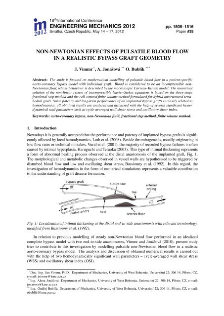
. 18m 2012th International ConferenceENGINEERING MECHANICS 2012 pp. 1505–1516Svratka, Czech Republic, May 14 – 17, 2012 Paper #38NON-NEWTONIAN EFFECTS OF PULSATILE BLOOD FLOWIN A REALISTIC BYPASS GRAFT GEOMETRYJ. Vimmr * , A. Jonášová ** O. Bublík ***Abstract: The study is focused on mathematical modelling of pulsatile blood flow in a patient-specificaorto-coronary bypass model with individual graft. Blood is considered to be an incompressible non-Newtonian fluid, whose behaviour is described by the macroscopic Carreau-Yasuda model. The numericalsolution of the non-linear system of incompressible Navier-Stokes equations is based on the three-stagefractional step method and the cell-centred finite volume method formulated for hybrid unstructured tetrahedralgrids. Since patency and long-term performance of all implanted bypass grafts is closely related tohemodynamics, all obtained results are analysed and discussed with the help of several significant hemodynamicalwall parameters such as cycle-averaged wall shear stress and oscillatory shear index.Keywords: aorto-coronary bypass, non-Newtonian fluid, fractional step method, finite volume method.1. IntroductionNowadays it is generally accepted that the performance and patency of implanted bypass grafts is significantlyaffected by local hemodynamics, Loth et al. (2008). Beside thrombogenesis, usually originating inlow flow rates or technical mistakes, Vural et al. (2001), the majority of recorded bypass failures is oftencaused by intimal hyperplasia, Haruguchi and Teraoka (2003). This type of intimal thickening representsa form of abnormal healing process observed at the distal anastomosis of the implanted graft, Fig. 1.The morphological and metabolic changes observed in vessel walls are hypothesised to be triggered bydisturbed blood flow and low and oscillating shear stress, Bassiouny et al. (1992). In this regard, theinvestigation of hemodynamics in the form of numerical simulations represents a valuable contributionto the understanding of graft disease formation.Fig. 1: Localisation of intimal thickening at the distal end-to-side anastomosis with relevant terminology,modified from Bassiouny et al. (1992).In relation to previous modelling of steady non-Newtonian blood flow performed in an idealizedcomplete bypass model with two end-to-side anastomoses, Vimmr and Jonášová (2010), present studytries to contribute to this investigation by modelling pulsatile non-Newtonian blood flow in a realisticaorto-coronary bypass model. The analysis and discussion of obtained numerical results is carried outwith the help of two hemodynamically significant wall parameters – cycle-averaged wall shear stress(WSS) and oscillatory shear index (OSI).* Doc. Ing. Jan Vimmr, Ph.D.: Department of Mechanics, University of West Bohemia, Univerzitní 22; 306 14, Pilsen; CZ,e-mail: jvimmr@kme.zcu.cz** Ing. Alena Jonášová: Department of Mechanics, University of West Bohemia, Univerzitní 22; 306 14, Pilsen; CZ, e-mail:jonasova@kme.zcu.cz*** Ing. Ondřej Bublík: Department of Mechanics, University of West Bohemia, Univerzitní 22; 306 14, Pilsen; CZ, e-mail:obublik@kme.zcu.cz

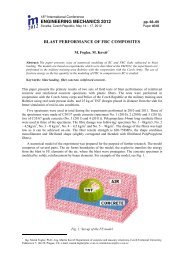
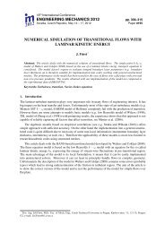
1506 Engineering Mechanics 2012, #382. Problem formulationThe main objective of this study is the analysis of hemodynamics in an individual aorto-coronary bypassgraft. In cardiovascular surgery, the term individual denotes a vascular graft with one distal end-to-sideanastomosis, i.e., the graft provides a direct connection between the aorta and the stenosed or occludedcoronary artery. The bypass model considered in this study is reconstructed from CT data provided by thecourtesy of the University Hospital in Pilsen, Czech Republic. The reconstruction process and computationalmesh generation are carried out in software packages Amira and Altair Hypermesh, respectively.An example of primary reconstruction of the chest region and of the individual bypass graft is shownin Fig. 2. The final shape of the bypass model after smoothing is displayed in Fig. 3. The unstructuredcomputational mesh used for all numerical simulations consists of 362,437 tetrahedral cells.Fig. 2: CT reconstruction of the chest region (left) and of the aorto-coronary bypass graft (right)For the purpose of blood flow simulations in the prepared individual graft, we choose an approachsimilar to that found in other studies published to the theme of bypass hemodynamics, see the reviewpaper Loth et al. (2008). Firstly, taking into account the fact that at the end of the arterialisation process,venous grafts lose their compliance, all the bypass walls are, in this study, modelled as impermeable andrigid, including the wall of the aorta. In the light of this simplification, we are aware that the neglectedaortic elasticity represents a considerable limitation of the present study. We hope to rectify it in one ofour future projects by solving the fluid-structure interaction problem. In this study, we further assume astatic aorto-coronary bypass model, i.e., the impact of heart beating is not considered. This assumptionis based on the findings published in Zeng et al. (2003), where it was shown that the arterial motiondoes not significantly affect blood flow in the case of flow pulsatility. In order to model blood’s complexrheological properties, we introduce the macroscopic non-Newtonian Carreau-Yasuda model, which wehave successfully applied in our previous simulations, Vimmr and Jonášová (2010),η( ˙γ) = η ∞ + (η 0 − η ∞ )[1 + ( λ ˙γ ) ] a n−1a, (1)where η 0 and η ∞ are the zero and infinite shear viscosities, respectively, λ is the characteristic relaxationtime and n is the flow index. The five parameters occurring in the Carreau-Yasuda model (1) maybe determined by numerical fitting of experimental data. In this study, we adopt data mentioned inCho and Kensey (1991): η ∞ = 3.45 · 10 −3 Pa · s, η 0 = 56 · 10 −3 Pa · s, λ = 1.902 s, a = 1.25,n = 0.22. The shear rate is given as ˙γ = 2 √ D II , where D II denotes the second invariant of the rate ofdeformation tensor D = 1 (2 ∇v + (∇v)T ) . For the incompressible fluid, the second invariant is definedas D II = 1 2 d ijd ij , i, j = 1, 2, 3, where d ij are the components of the rate of deformation tensor D. Forthe Newtonian flow, the molecular viscosity is kept constant and equal to infinite shear viscosity η ∞ .Finally, note that the coronary arteries shown in Fig. 3 are considered to be occluded (with no inflow) sothat the only relevant incoming flow will be that of the bypass graft.

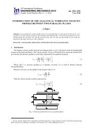
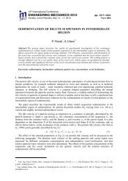
Vimmr J., Jonášová A., Bublík O. 1507Fig. 3: Individual graft – unstructured computational mesh and relevant terminology3. Mathematical modelLet us consider a time interval (0, T ), T > 0 and a bounded three-dimensional computational domainΩ ⊂ R 3 with boundary ∂Ω = ∂Ω I ∪ ∂Ω O ∪ ∂Ω W , where ∂Ω I , ∂Ω O and ∂Ω W denote the inlet, theoutlet and the walls of the computational domain, respectively. In this study, coronary blood flow ismodelled as unsteady laminar isothermal flow of incompressible generalised Newtonian fluid that in thespace-time cylinder Ω T = Ω × (0, T ) is mathematically described by the non-linear system of incompressibleNavier-Stokes (NS) equations written in the non-dimensional form∂v i= 0 , (2)∂x i∂v i∂t + ∂ (v i v j ) + ∂p = 1 [ (∂ ∂viη( ˙γ) + ∂v )]jfor i, j = 1, 2, 3 , (3)∂x j ∂x i Re ∂x j ∂x j ∂x iwhere t ∈ (0, T ) is the time, v i is the i-th component of the velocity vector v = [v 1 , v 2 , v 3 ] T correspondingto the Cartesian component x i of the space variables vector x = [x 1 , x 2 , x 3 ] T ∈ Ω, p is the pressure,Re is the reference Reynolds number and η( ˙γ) is the shear-dependent viscosity given by Eq. (1).All variables appearing in Eqs. (2) – (3) are non-dimensionalized by the reference velocity U ref > 0and characteristic length D ref > 0. For the bypass model considered in this study, the characteristiclength value was chosen to be equal to the aorta diameter D ref ≡ D (A) = 0.036 m and the referencevelocity is stated as U ref = 4Q 0 /(π Dref 2 ) = 0.1592 m · s−1 , where average aortic inlet flow rate isQ 0 = 112.56 · 10 −6 m 3 · s −1 , see Fig. 6 (left). As for the reference Reynolds number, it is determinedas Re = U ref D ref ϱ/η ref = 1 744.3, where ϱ = 1050 kg · m −3 and η ref ≡ η ∞ = 3.45 · 10 −3 Pa · s.For the sake of completeness, reference pressure and reference time are computed as p ref = ϱ Uref 2 andt ref = D ref /U ref , respectively.4. Numerical methodThe numerical solution of the non-linear time-dependent system of incompressible NS equations (2) –(3) is based on the projection method. In this study, the computation of velocity components vin+1 , whichsatisfy the divergence-free condition (2), employs the three-stage fractional step scheme, Ferziger andPerić (1999). In the first stage, intermediate velocity components vi ∗ are explicitly computed from theconvective part of the NS equation (3) asv ∗ i − vn i∆t+ ∂∂x j(v n i v n j ) = 0 , i, j = 1, 2, 3 . (4)

1508 Engineering Mechanics 2012, #38For the second stage of the fractional step scheme, the intermediate velocity components ˆv i are computedapplying the unconditionally stable implicit Crank-Nicolson scheme to the viscous term of Eq. (3)ˆv i − vi∗ = 1 [ (∂ ∂(ˆvi + vi ∗ η( ˙γ)) + ∂(ˆv j + vj ∗))], i, j = 1, 2, 3. (5)∆t 2Re ∂x j ∂x j ∂x iLet us linearise the shear-dependent dynamic viscosity η( ˙γ) as η( ˙γ) = η( ˙γ(v ∗ )) and introduce an auxil-(iary variable d ij = 1 ∂vi2 ∂x j+ ∂v j∂x i), which in this case is equal to the components of the rate of deformationtensor D mentioned in section 2. Then Eq. (5) can be rewritten as a system of two linear equationsˆv i − v ∗ i∆t= 1 ∂[ (η( ˙γ) ˆdij + dRe ∂xij)]∗ , (6)jˆd ij = 1 ( ∂ˆvi+ ∂ˆv )j. (7)2 ∂x j ∂x iIn the third stage, pressure is used for the projection of the intermediate velocity vector ˆv onto a spaceof divergence-free velocity field to get the values of velocity and pressure at the next time level (n + 1).Hence, the velocity components vin+1 are computed fromv n+1i− ˆv i∆twhere p n+1 is computed from the Poisson equation for pressure+ ∂pn+1∂x i= 0 , i = 1, 2, 3, (8)∂ 2 p n+1= 1 ∂ˆv i. (9)∂x i ∂x i ∆t ∂x iIt can be easily shown that sum of Eqs. (4), (5) and (8) yields the approximation of NS equations offirst order time accuracy. Finally, the whole algorithm of the fractional step method may be written fori, j = 1, 2, 3 as followsˆv i∆t − 1 Rev ∗ i∂(η( ˙γ)∂x ˆd)ijjˆd ij − 1 ( ∂ˆvi+ ∂ˆv )j2 ∂x j ∂x i= v n i − ∆t∂ 2 p n+1∂x i ∂x i= 1 ∆tv n+1i= v∗ i∆t + 1 Re∂ (vn∂x i v n )j , (10)j∂∂x j(η( ˙γ) d∗ij), (11)= 0 , (12)∂ˆv i∂x i, (13)= ˆv i − ∆t ∂pn+1∂x i. (14)The space discretization of the system of Eqs. (10) – (14) is performed using the cell-centred finitevolume method for hybrid unstructured tetrahedral grids. The idea of applying the hybrid unstructuredgrid for the numerical solution of time-dependent incompressible NS equations in 2D was introduced inKim and Choi (2000). The principle of this grid system lies in the coupling between an interpolationmethod, which will be described later, and the non-staggered grid system. Being inspired with this idea,we consider in this study a control volume Ω k in the form of tetrahedron, Fig. 4. The hybrid grid systemdefines the values of pressure and Cartesian velocity components in the centre of the control volume Ω kand the values of face-normal velocity V m , which has the direction of outward unit vector n m knormal tothe m-th face Γ m k of the control volume Ω k, is defined in the middle of the face Γ m k .After the integration of Eqs. (10) – (14) over each control volume Ω k , Fig. 4, k = 1, 2, . . . , N CV ,where N CV is the number of control volumes within the hybrid unstructured tetrahedral computationalmesh, after the introduction of integral average for an arbitrary flow quantity Φ over the control volumeΩ k(Φ) k = 1 ∫ΦdΩ, (15)|Ω k |Ω k

Vimmr J., Jonášová A., Bublík O. 1509Fig. 4: A tetrahedral control volume Ω k = A 1 A 2 A 3 A 4 with boundary ∂Ω k =hybrid unstructured computational mesh.⋃ 4 Γ m km=1belonging to thewhere |Ω k | is the volume of the tetrahedral control volume Ω k , and finally, after the application of theGauss-Ostrogradsky theorem, which converts the volume integrals to surface integrals, we get(vi ∗ ) k = (vi n ) k − ∆t ∮(vn|Ω k | j · jn )k · vni dΓ, (16)∂Ω k1∆t (ˆv i) k − 1 ∮η( ˙γ)Re|Ω k |ˆd ij · jn k dΓ = 1 ∆t (v∗ i ) k + 1 ∮η( ˙γ) d ∗ ij · jn k dΓ, (17)Re|Ω k |∂Ω k ∂Ω k⎛⎞( )ˆdij − 1 ∮⎜⎝ ˆv i · jn∮k dΓ + ˆv j · in ⎟k dΓ⎠ = 0 , (18)k 2∂Ω k ∂Ω k∮∂p n+1dΓ = 1 ∮ˆv i · in k dΓ, (19)∂n k ∆t∂Ω k ∂Ω k(vin+1 ) k = (ˆv i ) k − ∆t ∮p n+1 · in k dΓ, (20)|Ω k |∂Ω kwhere i n k is the i-th component of the outward unit vector n k = [ 1 n k , 2 n k , 3 n k ] T normal to the boundary∂Ω k of the tetrahedral control volume Ω k , Fig. 4. In order to achieve the satisfaction of the continuityequation for the normal velocity V = v i · in k , the system of Eqs. (16) – (20) is completed with followingequationV n+1 = ˆV − ∆t ∂pn+1∂n k. (21)This equation defines the normal velocity V n+1 at the time level (n + 1) having the direction of theoutward unit vector n k normal to the boundary ∂Ω k of the control volume Ω k . For the intermediatenormal velocity ˆV , it is valid that ˆV = ˆv i · in k .Further, we perform the approximation of surface integrals in the system of Eqs. (16) – (20). Firstly,each integral is replaced by the sum of integrals over each face Γ m kof the control volume Ω k, Fig. 4, and

1510 Engineering Mechanics 2012, #38then approximated by the midpoint rule∮Φ dΓ =∂Ω k4∑∫m=1Γ m k4∑Φ dΓ ≈ Φ m |Γ m k |, (22)m=1where |Γ m k |, m = 1, . . . , 4 is the area of the m-th face Γm kof the control volume Ω k and Φ m is the valueof an arbitrary flow quantity at the integration point at the same face. The interpolation process neededfor the determination of Φ m at the m-th face Γ m kof the control volume Ω k will be described later. UsingEq. (22), the system of Eqs. (16) – (21) is modified as follows(ˆv i ) k∆t(v ∗ i ) k = (v n i ) k − ∆t|Ω k |4∑m=1(V n m · v n i m| upwind)|Γ m k | , (23)14∑−η( ˙γ) m m ˆdRe |Ω k |ij · jn m k |Γm k | = (v∗ i ) k 14∑+η( ˙γ) m d ∗mij · jn m k∆t Re |Ωm=1k ||Γm k |, (24)m=1(( )4∑)ˆdij − 1 ˆv i m · jn4∑mkk 2| Γm k | + ˆv j m · in m k | Γm k | = 0 , (25)m=1m=14∑ ∂p n+1∂n m |Γ m k | = 1 4∑ˆv i m · in m km=1 k∆t| Γm k | ≡ 1 4∑ˆV m |Γ m k |, (26)∆tm=1m=1(vin+1 ) k = (ˆv i ) k − ∆t 4∑p n+1m · in m k|Ω k ||Γm k | , (27)V n+1mm=1= ˆV m − ∆t ∂pn+1∂n m k, (28)where i n m k is the i-th component of the outward unit vector nm k= [1 n m k , 2 n m k , 3 n m k ]T normal to the m-thface Γ m kof the control volume Ω k and for the intermediate face-normal velocity ˆV m at the m-th face Γ m kof the control volume Ω k , it is valid that ˆV m = ˆv im · in m k. Note that the values of face-normal velocityVmn+1 computed with the help of Eq. (28) are used as values of face-normal velocity Vm n in Eq. (23) atthe next time level.Explicit schemes are known for their disadvantage in the form of restricted time steps. The CFLstability condition imposed on the time step size becomes essential when it is applied for grids with largedifferences in cell size, e.g., in complex geometries. In this case, the efficiency of explicit schemes islost, since the cell with the most restrictive local time step determines the size of the global time step forall grid cells. One of possible solutions to this problem lies in the application of the well-known localtime-stepping method. This method, whose approach is also employed in our developed solver, enableseach cell of the computational grid to run with its own time step in a time-consistent manner.Interpolation methodTo perform numerical computations according to Eqs. (23) – (28), it is necessary to determine valuesof vi n m | upwind , ˆv i m, p n+1m and derivatives ∂ˆv i ∂v∂n m i,∗k ∂n m , ∂pn+1k ∂n m at the m-th face Γ m kof the control volumekΩ k . The value of vi n m | upwindis computed by the upwind scheme, whose first order accuracy is increasedby linear reconstruction with Barth’s limiter,v n i m| upwind={(vni ) L + σLBarth(vi n) R + σRBarth· ∂(vn i ) L∂x j· r jL , Vm n > 0 ,· ∂(vn i ) R∂x j· r jR , Vm n ≤ 0 ,(29)where σ Barth ∈ [0, 1] is the Barth’s limiter, Barth and Jesperson (1989), and vectors r L , r R are denotedin Fig. 5 (left). Further, the value Φ m of an arbitrary flow quantity Φ at the mid-point O of the m-thface Γ m k, Fig. 5 (right), can be stated with the help of second order accurate linear interpolation from

Vimmr J., Jonášová A., Bublík O. 1511values (Φ) k and (Φ) lm defined in cell-centres S k and S lm of two adjacent control volumes Ω k and Ω lm ,respectively,Φ m = (Φ) k + (Φ) l m− (Φ) kγ k + γ lm· γ k = γ l m(Φ) k + γ k (Φ) lmγ k + γ lm, (30)where γ k and γ lm are the minimal distances to the cell-face Γ m k from cell-centres S k and S lm of theadjacent control volumes Ω k and Ω lm , respectively, Fig. 5 (right). The derivative of flow quantity Φ inthe direction of the outward unit vector n m k normal to the m-th face Γm k of the control volume Ω k, isapproximated at the mid-point O of the face Γ m k, Fig. 5 (right), as∣∂Φ∂n m k∣∣Γ mk≈ (Φ) l m− (Φ) kγ k + γ lm. (31)A crucial part of the interpolation method is the application of Eq. (31) to the normal derivative inEqs. (26) and (28). In this way, it is ensured that the face-normal velocity Vmn+1 satisfies the continuityequation at the time level (n + 1) exactly, see Eq. (37). However, in general velocities (vin+1 ) k incell-centres of control volumes Ω k do not satisfy the continuity equation.Fig. 5: Definition of the vectors r L and r R for two adjacent tetrahedral control volumes Ω L and Ω R(left). Two adjacent tetrahedral control volumes Ω k = A 1 A 2 A 3 A 4 and Ω lm = A 1 A 2 A 3 A 5 with theircontact face Γ m k= ∆A 1A 2 A 3 (right).Regarding the implementation of non-dimensional boundary conditions at the boundary ∂Ω of thecomputational domain Ω ⊂ R 3 , three boundary types are considered in this study:• inlet Γ m k⊂ ∂Ω I – In this case, Dirichlet boundary conditions for the velocity components v i mand the auxiliary variable d m ij are prescribedv i m = v i I , d m ij · jn = 0. (32)The value of face-normal velocity Vm I at the face Γ m kis computed as V m I = v i I · in m k, where valuesv i I are given according to section 5. For the normal derivative of the pressure p n+1 at the face Γ m k ,we prescribe∂p n+1∂n m ∣ = 0. (33)k Γ mk• rigid and impermeable wall Γ m k ⊂ ∂Ω W – Velocity components v i m at the face Γ m kare set equalto zerov i m = 0 , (34)leading to zero value of the face-normal velocity Vm W = v i m · in m k = 0 at the face Γm k. For theauxiliary variable dij m , we apply the Dirichlet boundary condition in the following formd m ij · jn = 0 . (35)Further, zero normal derivative of the pressure p n+1 (33) is prescribed at the wall.

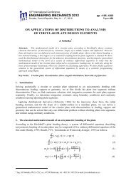
1512 Engineering Mechanics 2012, #38• outlet Γ m k⊂ ∂Ω O – Following type of boundary condition is statedp m n m k − 1 Re 2 η( ˙γ)m d m ij · jn m k = p On m k , (36)where p O is the given value of the outlet pressure, for details see section 5.Substituting the derivative ∂pn+1∂n m in Eq. (26) with Eq. (28), we getk4∑ ∂p n+1∂n m |Γ m k | = 1 4∑m=1 k∆tm=14∑=⇒m=1( )ˆVm − Vmn+1 |Γ m k | = 1 ∆t4∑m=1ˆV m |Γ m k |Vm n+1 |Γ m k | = 0, (37)i.e., face-normal velocities Vmn+1 satisfy the continuity equation exactly. At this point, let us mentionthat at the outlet boundary ∂Ω O , i.e., at the face Γ m k of the control volume Ω k, where Γ m k ⊂ ∂Ω O, values∂p n+1∂n m kare unknown. In order to ensure the satisfaction of the continuity equation (37) for this controlvolume Ω k , it is necessary to compute the face-normal velocity Vm n+1 at the face Γ m k ⊂ ∂Ω O asVm n+1O= − 1 4∑|Γ m VOm n+1 |Γ m k |, (38)k|m=1m≠m Owhere m O is the index of the outlet face Γ m Okof the control volume Ω k . For the whole computationaldomain Ω ⊂ R 3 at the time t = 0, following initial conditions are used(vi 0 ) k = 1 ∫v i (x, 0)dΩ = 0, (p 0 ) k = 1 ∫p(x, 0)dΩ = p initial , k = 1, 2, . . . , N CV ,|Ω k ||Ω k |Ω k Ω kwhere p initial is a non-dimensional value of static pressure.5. Numerical resultsIn accordance with the boundaries of the computational domain denoted in Fig. 3 for the model of theindividual aorto-coronary bypass, the numerical simulations of pulsatile Newtonian and non-Newtonianblood flow are carried out with following values of the time-dependent boundary conditions:• aortic inlet ∂Ω (A)I– constant time-dependent velocity profile |v I | according to the flow rate waveformQ(t) shown in Fig. 6 (left);• aortic outlet ∂Ω (A)O– time-dependent pressure p(t) shown in Fig. 6 (right), where the aortic pressureis plotted in the medical units of millimeters of mercury (1 mmHg = 133.333 Pa);• coronary outlets ∂Ω (CA)O– constant pressure related to average arterial pressure of 12 000 Pa;• rigid and impermeable walls ∂Ω W – non-slip boundary condition.Note that the boundary values mentioned above are, for the computation, non-dimensionalized using thereference values mentioned in section 3. The implementation of the boundary conditions in the numericalcode is described in detail in section 4.For the analysis of computed numerical results, we introduce two significant hemodynamical wallparameters – the cycle-averaged wall shear stress (WSS) and the oscillatory shear index (OSI) that areevaluated according to formulas mentioned in Xiong and Chong (2008) and He and Ku (1996), respectively,⎡|τ W | = 1 ∫ T|τ W |dt , OSI = 1 ∫⎢T ⎛∫ T ⎞⎣1 −T2τ W dt∣ ∣ · ⎝ |τ W |dt⎠−1 ⎤ ⎥ ⎦ , (39)0where |τ W | is the WSS magnitude and T = 1 s is the duration of one cardiac cycle, Fig. 6.00

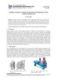
Vimmr J., Jonášová A., Bublík O. 1513450400350300Q(t) [ml/s]2502001501005000 0.2 0.4 0.6 0.8 1time [s]Fig. 6: Time-dependent boundary conditions for the aorta – inlet flow rate Q(t) (left) and outlet pressurep(t) (right), data taken from Olufsen et al. (2000)Firstly, let us analyse the velocity profiles of the non-Newtonian blood flow in Fig. 7 for three selectedtime instants, corresponding to systole, diastole and late diastole, respectively. During the systolic phase(t 1 = 0.16 s), Fig. 7 (left), the graft’s proximal anastomosis becomes exposed to the increased flow ratein the aorta. Although the skewed velocity profiles at the graft entrance may indicate incoming bloodflow, the real graft filling occurs later. By comparing the pictures in Fig. 7, it becomes quite apparentthat the systolic phase of the cardiac cycle is represented by decreased blood flow through the individualbypass graft, whereas an opposite effect is observed during most of the diastolic phase (t 2 = 0.47 s andt 3 = 0.98 s). In this case, the velocity increase observed along the individual graft is also accompaniedby skewed or otherwise shaped velocity profiles that are a result of the out-of-plane geometry and thegraft’s winding around the heart, see Fig. 2. At the distal end-to-side anastomosis, Fig. 7c, the incomingblood flow seems to prefer the closer branch of the coronary artery more than the second one. Moreover,the closer coronary artery shows a tendency to considerably increase velocity magnitude downstreamfrom the anastomosis. The reason for this phenomenon is a partly stenosed coronary artery.The comparison between the Newtonian and non-Newtonian blood flow is illustrated by the distributionsof the cycle-averaged WSS and OSI in Figs. 8 and 9, respectively. At this point, note thelowered value range in Fig. 8, which is chosen according to conclusions mentioned in Haruguchi andTeraoka (2003) and He and Ku (1996). Namely, that low WSS, as compared to the normal range between1 − 2 Pa in healthy arteries, is one of the confirmed triggers of vessel remodelling, plaque growthand intimal thickening. In light of this fact, we will further assess the resulting shear distribution, whichregardless of the viscosity model (Newtonian or non-Newtonian), seems to be non-uniform at both anastomoses,Fig. 8. One of the distinct areas with extremely low shear is situated at the entrance of thegraft, where it is caused by a large recirculation zone that is present there most of the cardiac cycle. Thisnegative stimulation of the proximal suture line is also confirmed by the high OSI shown in Fig. 9. At thedistal anastomosis, shear values below 1 Pa are observed at the heel and the arterial floor in accordancewith the sites of intimal hyperplasia displayed in Fig. 1. In this case, the critical shear stress also showsa oscillatory tendency as is apparent from the OSI distribution in Fig. 9.The objective of our previous study, Vimmr and Jonášová (2010), was the investigation of blood’snon-Newtonian behaviour in complete bypass models with coronary or femoral native arteries. Thenumerical simulations were carried out under steady flow conditions and for an idealized bypass geometry.In the present study, we want to extend our previous conclusions about the importance of blood’snon-Newtonian modelling in coronary bypasses by considering pulsatile blood flow and a realistic andmore complex bypass geometry. As is illustrated by Figs. 8 – 9, the influence of non-Newtonian flowconditions is very small or rather negligible (as is the case of the velocity profiles). On the basis ofthese observations, we can draw a conclusion similar to that mentioned in Vimmr and Jonášová (2010).Namely, that blood’s non-Newtonian behaviour does not have any significant impact on the hemodynamicsin coronary bypasses. In light of this observation and our present experience with the modellingof non-Newtonian blood flow, it may be said that an hemodynamic study in patient-specific femoral bypasseswould be more promising in regard to the occurrence of non-Newtonian effects as was concludedin our previous study Vimmr and Jonášová (2010). This problem will be addressed in the future.

1514 Engineering Mechanics 2012, #38Fig. 7: Non-Newtonian blood flow – velocity profiles at selected cross-sections of the aorto-coronary bypass at the time instants t1 = 0.16 s, t2 = 0.47 s andt3 = 0.98 s (from left to right); detailed views at (a) the proximal anastomosis, (b) individual graft, (c) coronary arteries with the distal anastomosis

Vimmr J., Jonášová A., Bublík O. 1515Fig. 8: Distribution of cycle-averaged WSS for the Newtonian (left) and non-Newtonian flow (right)Fig. 9: Distribution of OSI for the Newtonian (left) and non-Newtonian flow (right)

1516 Engineering Mechanics 2012, #38AcknowledgmentsThis study was supported by the European Regional Development Fund (ERDF), project NTIS - NewTechnologies for Information Society, European Centre of Excellence, CZ.1.05/1.1.00/02.0090 and bythe internal student grant project SGS-2010-046 of the University of West Bohemia.ReferencesBassiouny, H.S., White, S., Glagov, S., Choi, E., Giddens, D.P., Zarins, C.K. (1992), Anastomotic intimal hyperplasia:Mechanical injury or flow induced. Journal of Vascular Surgery, Vol 15, No.4, pp 708-717.Barth, T.J., Jesperson, D.C. (1989), The design and application of upwind schemes on unstructured meshes. In:Proceedings of the 27th AIAA Aerospace Sciences Meeting. AIAA Paper 89-0366.Cho, Y.I., Kensey, K.R. (1991), Effects of the non-Newtonian viscosity of blood on flows in diseased arterialvessels. Part I: Steady flows. Biorheology, Vol 28, No.3-4, pp 241-262.Ferziger, J.H., Perić M. (1999), Computational methods for fluid dynamics, Springer, Heidelberg.Haruguchi, H., Teraoka, S. (2003), Intimal hyperplasia and hemodynamic factors in arterial bypass and arteriovenousgrafts: A review. Journal of Artificial Organs, Vol 6, No.4, pp 227-235.He, X., Ku, D.N. (1996), Pulsatile flow in the human left coronary artery bifurcation: Average conditions. Journalof Biomechanical Engineering, Vol 118, No.1, pp 74-82.Kim, D., Choi, H. (2000) A second-order time accurate finite volume method for unsteady incompressible flow onhybrid unstructured grids. Journal of Computational Physics, Vol 162, No.2, pp 411-428.Loth, F., Fischer, P.F., Bassiouny, H.S. (2008) Blood flow in end-to-side anastomoses. Annual Review of FluidMechanics, Vol 40, pp 367-393.Olufsen, M.S., Peskin, C.S., Kim, W.Y., Pedersen, E.M., Nadim, A., Larsen, J. (2000) Numerical simulation andexperimental validation of blood flow in arteries with structured-tree outflow conditions. Annals of BiomedicalEngineering, Vol 28, No.11, pp 1281-1299.Vimmr, J., Jonášová, A. (2010), Non-Newtonian effects of blood flow in complete coronary and femoral bypasses.Mathematics and Computers in Simulation, Vol 80, No.6, pp 1324-1336.Vural, K.M., Şener, E., Taşdemir, O. (2001) Long-term patency of sequential and individual saphenous vein coronarybypass grafts. European Journal of Cardio-thoracic Surgery, Vol 19, No.2, pp 140-144.Xiong, F.L., Chong, C.K. (2008), A parametric numerical investigation on haemodynamics in distal coronaryanastomoses. Medical Engineering & Physics, Vol 30, No.3, pp 311-320.Zeng, D., Ding, Z., Friedman, M.H., Ethier, C.R. (2003), Effects of cardiac motion on right coronary arteryhemodynamics. Annals of Biomedical Engineering, Vol 31, No.4, pp 420-429.