Numerical Differentiation

Numerical Differentiation 

● 

● 

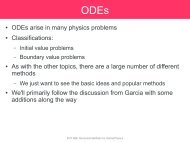
We'll follow the discussion in Pang (Ch. 3) with some additions 

along the way 

Numerical differentiation approximations are key for: 

– Solving ODEs 

– PDEs 

PHY 688: Numerical Methods for (Astro)Physics

Numerical Differentiation 

● 

We can imagine 2 situations 

– We have our function f(x) defined only at a set of (possibly 

regularly spaced) points 

● 

Generally speaking, asking for greater accuracy involves using 

more of the discrete points in the approximation for f' 

– We have an analytic expression for f(x) and want to compute the 

derivative numerically 

● 

● 

Usually it would be better to take the analytic derivative of f(x), but 

we can learn something about error estimation in this case. 

Used, for example, in computing the numerical Jacobian for 

integrating a system of ODEs (we'll see this later) 


Gridded Data 

● 

Discretized data is represented at a finite number of locations 

– Integer subscripts are used to denote the position (index) on the 

grid 

– Structured/regular: spacing is constant 

– Data is known only at the grid points: 


First Derivative / Order of Accuracy 

● 

Taylor expansion: 

● 

Solving for the first derivative: 

Discrete approximation to 

Leading term in the 

truncation error 



● 

● 

This is a first-order accurate expression for the derivative at 

point i 

– Alternately, we can use the point to the left (blackboard) 

– The are called difference or finite-difference formulae 

Shorthand: 

– “big-O notation” 

● 

How can we get higher order 



● 

First derivative approximations: 

– First-order (one-sided): 

2-point stencil 

– Second-order (centered): 


– Fourth-order: 


● 

Range of points involved is called the stencil 

– Some points may have a '0' coefficient 



● 

● 

● 

General trend: more points = higher accuracy 

– Found via Taylor expanding from greater distances and algebra 

What happens at the boundaries of our finite-gridded data 

– Can interpolate past the last point to use the same stencil 

– Can switch to one-sided stencils 

Practically speaking: the first and second order approximations 

are the ones that are used the most often. 


First Derivative Comparison 

analytic: 0.5 

left-sided O(dx): 0.639529171481 

right-sided O(dx): 0.34028636457 

centered O(dx**2): 0.489907768026 

centered O(dx**4): 0.499756119208 


Roundoff vs. Truncation Error 

(Yakowitz & Szidarovszky) 

● 

Just evaluating f at our gridded points introduces round-off 

error: 

– is an approximation to 

– Assume some bound: 

– Error is (blackboard): 

This should be 

near machine ε 

truncation 

roundoff 

As ¢ x → ε, the 

roundoff term 

becomes O(1) 

Another thing to consider: with roundoff, is 


Round-off vs. Truncation Error 

● 

exp(x) 


Higher-Derivatives 

● 

Graphically 

This is 2 nd order at the midpoint between 

the two points 

This is a centered difference (derivative) of 

the derivatives = second derivative 

Second-order accurate 

● 

Also via Taylor expansion (blackboard) 


Non-Uniform Data 

● 

Two choices: 

– Interpolate to a uniform grid 

– Re-derive our expressions for a non-uniform grid (preferred) 

(blackboard derivation...) 


Analytic f Given 

● 

● 

If we have f(x) available analytically, we can make estimates of 

the error 

– This will come into play with ODEs, where we have the analytic 

righthand side 

Controlling accuracy 

– Consider: 

– We are free to choose h 

– Compare to estimate error 


Analytic f Given 

● 

Iteratively build more accurate approximations 

– 

– This gives: 

– Consider: 

– Combine: 

– This is an example of Richardson extrapolation—we'll see this 

more when we go to ODEs 


Numerical Integration 

● 

We want to solve: 

● 

● 

Again, we have two distinct cases: 

– f(x) is provided at discrete points on a grid 

– We have an analytic expression for f(x) 

We'll follow the discussion in Pang and also that of Garcia 



● 

Simplest case: piecewise constant interpolant (midpoint rule) 



● 

One step up: piecewise linear interpolant (trapezoid rule) 

This is just the area 

of a trapezoid 



● 

● 

As you might expect, the accuracy gets better the higher-order 

the interpolating polynomial 

– Trapezoid rule will integrate a linear f(x) perfectly 

What about a parabola 

– For now, we'll stick with equally spaced locations at which we 

evaluate f(x) 


Simpson's Rule 

● 

Piecewise linear interpolant (Simpson's rule) 

– 3 unknowns (A, B, C) and 3 

points 

– Blackboard algrebra... 


Simpson's Rule 

● 

Then integrate under the parabola 


Summary of Simple Rules 

(Yakowitz & Szidarovszky) 

● 

Error estimates 

– Actually rather complicated to derive (see a math text on 

Numerical Methods) 

– Simple trapezoidal: 

– Simple Simpson's: 

– Note the only way to reduce the error here is to make [a, b] 

smaller 

– Here, is some unknown point in [a, b] 


Summary of Simple Rules 

● 

● 

Any numerical integration method that represents the integral 

as a (weighted) sum at a discrete number of points is called a 

quadrature rule 

Fixed spacing between points (what we've seen so far): 

Newton-Cotes quadrature 


Open Integration Rules 

● 

Forms of these exist where the end-points of the interval are 

not used—these are open integration rules 

– Usually not very desirable 

– See, for example, Numerical Recipes 


Compound Integration 

● 

● 

Mid-point, trapezoidal, and Simpson's integration as we wrote 

them are ok when [a,b] is small. 

Integrating over large domain is not very accurate 

– We could keep adding terms to our polynomials (getting higher 

and higher degree), or we could string together our current 

expressions 

● 

More points = more accuracy 

– Compound integration—break domain into sub-domains and use 

these rules in each sub-domain. 



● Break interval into chunks 

Integral over a 

single slab 



● 

Compound Trapezoidal 

● 

Compound Simpson's 

– Integrate pairs of slabs together (requires even number of slabs) 



Always a good idea to check the convergence rate! 


Adaptive Integration 

● 

If you know the analytic form of f(x), then you can estimate the 

error by increasing N 

– Can make use of previous function evaluations (see Garcia) 

● 

Recover Simpson's rule from adaptive trapezoidal (see NR) 


Gaussian Quadrature 

● 

Instead of fixed spacing, what if we strategically pick the 

spacings 

– We want to express 

– w's are weights. We will choose the location of points x i 



(Garcia, Ch. 10) 

● 

Gaussian quadrature: fundamental theorem 

– q(x) is a polynomial of degree N, such that 

– k = 0, ..., N-1 and ρ(x) is a specified weight function. 

– Choose x 1 

, x 2 

, ... x N 

as the roots of the polynomial q(x) 

– We can write 

and there will be a set of w's for which the integral is exact if f(x) 

is a polynomial of degree < 2N! 




● 

● 

The amazing result of this theorem is that by picking the points 

strategically, we are exact for polynomials up to degree 2N-1 

– With a fixed grid, of N points, we can fit an N-1 degree 

polynomial 

● 

Exact integration for f(x) only if it is a polynomial of degree N-1 or 

less 

– If our f(x) is closely approximated by a polynomial of degree 2N- 

1, then this will be very accurate. 

Many choices of weighting function, ρ(x), leading to different 

q's and x's and w's. 




● 

Example from Garcia: 

– 3-point quadrature 

● 

This means 3 roots, so q(x) is a cubic 

– Weight function ρ(x) = 1 

– Work in the interval [-1, 1] 

● Easy to transform from [a, b] to [-1, 1]: 




● 

● 

3-point quadrature: 

– 

Step 1: Apply the theorem to find the c's: 

This can give 3 equations for the c's, 

allowing us to find q(x) up to some 

arbitrary factor. 

Alternately, these are the conditions for 

the Legendre polynomials (the Gram- 

Schmidt orthogonalization) 




● 

Step 2: find the roots (those are our quadrature points) 

– For 

we can easily factor this: 

– This means that our quadrature becomes: 




● 

Step 3: find the weights 

– The theorem tells us that with the x's as the roots, then the 

proper choice of weights makes the integration exact for 

polynomials up to degree 2N-1 

this is: 

Note the “=”—this is exact 




– These three equations can be solved to find the weights: 

● 

Therefore, our 3-point quadrature is: 

Our choice of weight function and integration interval results in 

the Gauss-Legendre method 



● Example: 


erf(1) (exact): 0.84270079295 

3-point trapezoidal: 0.825262955597 -0.017437837353 

3-point Simpson's: 0.843102830043 0.000402037093266 

3-point Gauss-Legendre: 0.842690018485 -1.0774465204e-05 

Notice how well the Gauss-Legendre does for this integral. 



● 

Other quadratures exist: 

(Wikipedia) 

● 

In practice, the roots and weights are tabulated for these out to 

many numbers of points, so there is no need to compute them. 


Multi-dimensional Integration 

● 

For multi-dimensional integration, Monte Carlo methods may 

be faster (less function evaluations)

Numerical Differentiation

Create successful ePaper yourself

Delete template?

Save as template?