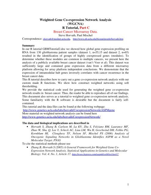
Weighted Gene Co-expression Network Analysis (WGCNA) R ...

Weighted Gene Co-expression Network Analysis 

(WGCNA) 

R Tutorial, Part C 

Breast Cancer Microarray Data. 

Steve Horvath, Paul Mischel 

Correspondence: shorvath@mednet.ucla.edu, http://www.ph.ucla.edu/biostat/people/horvath.htm 

Summary 

In our R tutorial GBMTutorial2.doc we showed how global gene expression profiling on 

RNA from 130 glioblastoma patient samples (dataset 1, n=55,15 and dataset 2, n=65) 

resulted in the identification of groups of highly coexpressed genes (modules). To 

determine whether these modules are common to multiple cancers, we present here the 

analysis of a publicly available breast cancer dataset (van’t Veer et al). This dataset was 

sufficiently large and contained gene expression data from a different microarray 

platform allowing for array platform independent conclusions. We demonstrate that the 

expression of intramodular hub genes inversely correlates with cancer recurrence in the 

breast cancer data 

This R tutorial describes how to carry out a gene co-expression network analysis with our 

custom made R functions. We show how construct weighted networks using soft 

thresholding. 

We provide the statistical code used for generating the weighted gene co-expression 

network results in breast cancer. Thus, the reader be able to reproduce all of our findings. 

This document also serves as a tutorial to weighted gene co-expression network analysis. 

Some familiarity with the R software is desirable but the document is fairly selfcontained. 

This tutorial and the data files can be found at the following webpage: 

http://www.genetics.ucla.edu/labs/horvath/CoexpressionNetwork/ASPMgene 

More material on weighted network analysis can be found here 

http://www.genetics.ucla.edu/labs/horvath/CoexpressionNetwork/ 

The data and biological implications are described in 

• Horvath S, Zhang B, Carlson M, Lu KV, Zhu S, Felciano RM, Laurance MF, 

Zhao W, Shu, Q, Lee Y, Scheck AC, Liau LM, Wu H, Geschwind DH, Febbo PG, 

Kornblum HI, Cloughesy TF, Nelson SF, Mischel PS (2006) Analysis of 

Oncogenic Signaling Networks in Glioblastoma Identifies ASPM as a Novel 

Molecular Target. PNAS 

To cite the statistical methods please use 

• Zhang B, Horvath S (2005) A General Framework for Weighted Gene Co- 

Expression Network Analysis. Statistical Applications in Genetics and Molecular 

Biology: Vol. 4: No. 1, Article 17. http://www.bepress.com/sagmb/vol4/iss1/art17 

1

Data 

We used the published data set from the breast cancer study by van ‘t Veer et al. 

(2002). We eliminated BRCA positive patients from the analysis since our interest was in 

investigating patients with BRCA negative risk profile. This resulted in 78 primary breast 

cancer patients. When carrying out an unsupervised clustering analysis involving the 

5000 most varying genes, we found that sample 54 in the original data set was an array 

outlier. Since network analysis is susceptible to such outliers, we removed it from the 

analysis and ended up with 77 array samples (patients). As binary clinical outcome we 

considered cancer recurrence within 5 years. 34 patients developed distant metastases 

within 5 years, and 44 remained disease-free after a period of at least 5 years. 

From each patient, 5 µg total RNA was isolated from snap-frozen tumour material 

and used to derive complementary RNA (cRNA). A reference cRNA pool was made by 

pooling equal amounts of cRNA from each of the sporadic carcinomas. Two 

hybridizations were carried out for each tumour using a fluorescent dye reversal 

technique on microarrays containing approximately 25,000 human genes synthesized by 

inkjet technology. Fluorescence intensities of scanned images were quantified, 

normalized and corrected to yield the transcript abundance of a gene as an intensity ratio 

with respect to that of the signal of the reference pool. We used the log10ratios provided 

by the original study as gene expression index. This is why this patient was dropped from 

our analysis. 

Probe sets that were common to both array platforms (GBM data and breast cancer) were 

mapped, and Pearson correlations for all gene pairs found in glioblastoma were 

recalculated in the breast cancer dataset. To determine which glioblastoma modules were 

preserved in the breast cancer data, we assigned the glioblastoma module colors to the 

genes in the hierarchical clustering tree of the breast cancer data. 

References 

't Veer,L.J., Dai,H., van de Vijver,M.J., He,Y.D., Hart,A.A., Mao,M., Peterse,H.L., van 

der,K.K., Marton,M.J., Witteveen,A.T., Schreiber,G.J., Kerkhoven,R.M., Roberts,C., 

Linsley,P.S., Bernards,R., and Friend,S.H. (2002). Gene expression profiling predicts 

clinical outcome of breast cancer. Nature 415, 530-536. 

Andy M. Yip and Steve Horvath (2006) “Generalized Topological Overlap 

Matrix and its Applications in Gene Co-expression Networks”, BIOCOMP'06 and 

WORLDCOMP'06 in Las Vegas. 

2

# R CODE 

#copy and past the following code into the R session 

# Please adapt the paths in the following. Make sure to use / instead of \ 

setwd(“C:/Documents and Settings/shorvath/My 

Documents/ADAG/PaulMischel/GBMnetworkpaper/Webpage/BreastCancerTutorial2”) 

source(“C:/Documents and Settings/shorvath/My 

Documents/RFunctions/NetworkFunctions.txt”) 

#Memory 

# check the maximum memory that can be allocated 

memory.size(TRUE)/1024 

# increase the available memory 

memory.limit(size=4000) 

sum1=function(x) sum(x,na.rm=T) 

#Quote: 

#"When popular opinion is nearly unanimous, contrary thinking tends to be most profitable. The 

reason is that once the crowd takes a position, it creates a short-term, self-fulfilling prophecy. But 

when a change occurs, everyone seems to change his mind at once." 

The Crowd - Gustave Le Bon 

3

Mapping Affymetrix U133a arrays (GBM) data into Rosetta Arrays 

(breast cancer) 

First we show how me mapped the 8000 most varying probes in the GBM samples 

(Affymetrix U133a) into the breast cancer data (Rosetta arrays) 

# This data sets contains the breast cancer expression data 

#and corresponding clinical traits 

dat1=read.csv(“BreastArrayDataCombined.csv”,header=T) 

datGenes=dat1[-c(1:5),] 

datClinicalBreast=dat1[1:5,] 

# There are 2 types of gene expression indices: intensity and ratio 

# We prefer the ratio... 

IndexIntensity=seq(from=2,to=233,by=3) 

IndexRatio=seq(from=3,to=234,by=3) 

names(datGenes[, IndexIntensity]) 

names(datGenes[, IndexRatio]) 

# This file contains gene information on the 

datGBM=read.csv(“GBM8000Summarydat55dat65.csv”) 

name1=row.names(dat1) 

# these tables will allow us to translate U133A Affymetrix probe set IDs into Rosetta IDs 

datAffy= read.csv(“AffyChip.csv”) 

datRosetta=read.csv(“RosettaChip.csv”) 

table(is.element(datGenes$Systematic_name, datRosetta$NAME)) 

table(is.element(datAffy$MEGID, datRosetta$MEGID)) 

table(is.element(datAffy$MEGACCESSOR, datRosetta$MEGACCESSOR)) 

table(is.element(datGBM$gbm133a,datAffy$NAME)) 

# Step 1: merge the GBM data with the folw datAffy, so that we get the MEG_IDs 

datmerge=merge(datGBM, datAffy , by.x=”gbm133a”, by.y= “NAME”) 

dim(datGBM) 

dim(datmerge) 

table(is.element(datmerge$MEGACCESSOR, datRosetta$MEGACCESSOR)) 

4

# Step 2: merge the datmerge with datRosetta by MEG_ACCESSOR so that 

# we get the Rosetta$NAME for each gene 

datmerge=merge(datmerge, datRosetta , by.x=”MEGACCESSOR”, 

by.y=“MEGACCESSOR”, all=FALSE) 

dim(datmerge) 

# The reason why we end up with a number different from 6569 rows is that the entries of 

# MEGACCESSOR are not unique, i.e. some are repeated. But this does 

# not lead to major trouble as seen below 

#Step 3 merge datmerge with the breast cancer data 

datmerge=merge(datmerge, datGenes, by.x=”NAME”, by.y=”Systematic_name”) 

table(datmerge$colordata1) 

blue brown green grey turquoise yellow 

660 180 145 5747 1438 156 

#Note that the number of genes per module is very close to that in the orignal data (see 

#below) especially for the brown module. 

table(datGBM$colordata1) 

blue brown green grey turquoise yellow 

618 167 140 5574 1352 149 

names(datmerge) 

# Since we focus on the ratio measurement for expression, we define 

IndexRatio=seq(from=24,to=255,by=3) 

names(datmerge[,IndexRatio]) 

# Whole Network Analysis 

datExpr=data.frame( t(datmerge[,IndexRatio])) 

names(datExpr)=datmerge[,1] 

names(datClinicalBreast) 

IndexRatio2=seq(from=3,to=234,by=3) 

datClinicalBreast2=datClinicalBreast[,IndexRatio2] 

table(names(datClinicalBreast2)==dimnames(datExpr)[[1]]) 

5

# the following shows that sample 54 is an outlier that will be removed below 

h1=hclust(dist(datExpr), method=”average”) 

plot(h1) 

Cluster Dendrogram 

Height 

10 20 30 40 50 60 

S54_Log10.ratio. 







































































dist(datExpr) 

hclust (*, "average") 

# Note that array number 54 appears to be an outlier. To be safe we remove it from the 

#analysis. Since dropping this array is done without reference to the clinical outcome, 

#this does not bias our result. 

dimnames(datExpr)[[1]] 

datExpr2=datExpr[-54,] 

dim(datExpr2) 

datClinicalBreast3=datClinicalBreast2[,-54] 

FiveYearRecurrence= as.numeric(as.vector(as.matrix(datClinicalBreast3[1,]))) 

RecurrenceFreeTime= as.numeric(as.vector(as.matrix(datClinicalBreast3[5,]))) 

table(FiveYearRecurrence) 

FiveYearRecurrence 

0 1 

33 44 

#Quote: 

#Until the day when God shall deign to reveal the future to man, 

#all human wisdom is summed up in these two words,--'Wait and hope'. 

#Alexandre Dumas, The Count of Monte Cristo 

6

#The following plot shows a close relationship between recurrence time and status. 

recurrence time 

0 50 100 150 

0 1 

Five year recurrence status 

rm(datExpr) 

rm(dat1) 

rm(datGBM) 

collect_garbage() 

7

# Now we define the connectivity (degree) in the breast network 

# We use the following power for the power adjacency function. 

beta1=6 


DegreeBreast= SoftConnectivity(datExpr2,power=beta1) 


ScaleFreePlot1(DegreeBreast,AF1=”Check Scale Free Topology in Breast CA”) 

Check Scale Free Topology in Breast CA , scale R^2= 0.9 , slope= -2.18 

log10(p(k)) 

-3.0 -2.5 -2.0 -1.5 -1.0 -0.5 

0.6 0.8 1.0 1.2 1.4 1.6 

log10(k) 

# Quote 

#As an adolescent I aspired to lasting fame, I craved factual certainty, and I thirsted for a 

meaningful vision of human life - so I became a scientist. This is like becoming an archbishop so 

you can meet girls. 

- M. Cartmill 

8

# This code allows one to restrict the analysis to the most connected genes, 

# which may speed up calculations when it comes to module detection. 

DegCut =3000 # number of most connected genes that will be considered 

DegreeRank = rank(-DegreeBreast) 

restDegree = DegreeRank

#Analysis of the brown (mitosis) module 

datExprbrown= datExpr2[,datmerge$colordata1==”brown”] 

#To ensure that the entries of datExprbrown are considered as numeric, we have to run 

#the following code. 

for (i in c(1:dim(datExprbrown)[[2]]) ) { 

datExprbrown[,i]=as.numeric(as.character(datExprbrown[,i])) 

} 

# This is the intramodular connectivity in the brown module 

kbrownBreast= SoftConnectivity( datExprbrown , beta1) 

# The following function determines the geme significance of a gene expresssion profile 

#based on its association with the breast cancer recurrence time. 

#Specifically, we first compute the p-value of the Spearman correlation between 

#recurrence time and a gene expression profile. 

# Then the gene significance is defined as the minus log10 of the p-value. 

# Roughly speaking, this measure counts the zeroes in the p-value. 

# If a gene has fewer than 6 measurements, its gene significance is set to missing 

if (exists(“corTime”) ) rm(corTime); 

corTime=function(x) { 

if( sum(!is.na(x) )

par(mfrow=c(1,2)) 

#Figure 2c 

scatterplot1(kbrownBreast, 

datmerge$kBrowndata1[datmerge$colordata1==”brown”],xlab1=”Connectivity (k)- 

Breast CA”, ylab1=” Connectivity (k)-GBM”,col1=”brown”) 

# This is Figure 2d in our article. 

scatterplot1( kbrownBreast, abs(GSBREAST),ylab1=”Recurrence Association: |Z|” 

,xlab1=”Connectivity (k)-Breast CA”,col1=”brown”) 

cor= 0.62 p= 1.9e-20 

cor= 0.7 p=

# The following figures are also interesting 

scatterplot1(kbrownBreast, 

datmerge$kBrowndata2[datmerge$colordata1==”brown”],xlab1=”K.intra, Breast 

Cancer”, ylab1=”K.intra Brain Cancer 65”,col1=”brown”) 

scatterplot1(-log10(datmerge$pCoxdata1[datmerge$colordata1==”brown”]), 

abs(GSBREAST),ylab1=”Breast CA RecurAssociation” 

,xlab1=”GBM prognostic significance”, col1=”brown”) 

cor= 0.54 p= 3.9e-15 

cor= 0.65 p=

Weighted Gene Co-expression Network Analysis (WGCNA) R ...

You also want an ePaper? Increase the reach of your titles

Delete template?

Save as template?