Weighted Gene Co-expression Network Analysis - UCLA
Weighted Gene Co-expression Network Analysis - UCLA
Weighted Gene Co-expression Network Analysis - UCLA

Create successful ePaper yourself
Turn your PDF publications into a flip-book with our unique Google optimized e-Paper software.
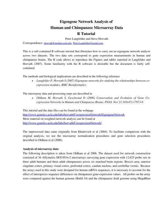
Eigengene <strong>Network</strong> <strong>Analysis</strong> ofHuman and Chimpanzee Microarray DataR TutorialPeter Langfelder and Steve Horvath<strong>Co</strong>rrespondence: shorvath@mednet.ucla.edu, Peter.Langfelder@gmail.comThis is a selfcontained R software tutorial that illustrates how to carry out an eigengene network analysisacross two datasets. The two data sets correspond to gene <strong>expression</strong> measurements in human andchimpanzee brains. The R code allows to reproduce the Figures and tables reported in Langfelder andHorvath (2007). Some familiarity with the R software is desirable but the document is fairly selfcontained.The methods and biological implications are described in the following reference• Langfelder P, Horvath S (2007) Eigengene networks for studying the relationships between co<strong>expression</strong>modules. BMC BioinformaticsThe microarray data and processing steps are described in• Oldham M, Horvath S, Geschwind D (2006) <strong>Co</strong>nservation and Evolution of <strong>Gene</strong> <strong>Co</strong><strong>expression</strong><strong>Network</strong>s in Human and Chimpanzee Brains. PNAS. Nov 21;103(47):179738This tutorial and the data files can be found at the webpagehttp://www.genetics.ucla.edu/labs/horvath/<strong>Co</strong><strong>expression</strong><strong>Network</strong>/Eigengene<strong>Network</strong>More material on weighted network analysis can be found athttp://www.genetics.ucla.edu/labs/horvath/<strong>Co</strong><strong>expression</strong><strong>Network</strong>/The unprocessed data came originally from Khaitovich et al (2004). To facilitate comparison with theoriginal analysis, we use the microarray normalization procedures and gene selection proceduresdescribed in Oldham et al (2006).<strong>Analysis</strong> of microarray dataThe following description is taken from Oldham et al 2006. The dataset used for network constructionconsisted of 36 Affymetrix HGU95Av2 microarrays surveying gene <strong>expression</strong> with 12,625 probe sets inthree adult humans and three adult chimpanzees across six matched brain regions: Broca's area, anteriorcingulate cortex, primary visual cortex, prefrontal cortex, caudate nucleus, and cerebellar vermis. Becausethe arrays used in this study were designed for human mRNA sequences, it is necessary to account for theeffect of interspecies sequence differences on chimpanzee gene<strong>expression</strong> values. All probes on the arraywere compared against the human genome (Build 34) and the chimpanzee draft genome using MegaBlast
(http://www.ncbi.nlm.nih.gov/BLAST/). Any probe without a perfect match in both species(approximately 1/4) was masked during the calculation of <strong>expression</strong> values (GCOSv1.2, Affymetrix,Inc). In addition, only probe sets with six or more matching probes were retained for subsequent analyses(n=11,768/12,625). For each array, <strong>expression</strong> values were scaled to an average intensity of 200(GCOSv1.2, Affymetrix, Inc.). Quantile normalization was then performed and interarray correlationswere calculated using R. Following quantile normalization, the average interarray correlation was 0.924among all 18 human arrays and 0.937 among all 18 chimpanzee arrays. In specific instances in which thecomposition of this dataset was altered, the removal of a brain region(s) took place prior to quantilenormalization.For computational reasons, network analysis was limited to 4000 probe sets. (Note: although some genesare represented by multiple probe sets and other probe sets are not fully annotated, for consistency werefer to probe sets as "genes" throughout the manuscript, unless otherwise noted.) In order to enrich thissubset with genes likely to play important roles in the brain, a nonneural "filter" was applied to identifygenes with greater variance in neural versus nonneural tissue. A publicly available microarray datasetwas obtained for human lung (3). The human lung dataset consisted of 18 Affymetrix HGU95Av2microarrays measuring gene <strong>expression</strong> in normal adult human lung tissue, and was normalized asdescribed above. The same probe mask file that was used for the human and chimpanzee brain datasetswas also applied to the human lung dataset. After scaling all arrays to the same average intensity (200),the mean interarray correlation for one human lung array (CL2001032718AA) was 2.91 SD below theaverage and was removed from the dataset. Following quantile normalization in R, the average interarraycorrelation for the human lung dataset was 0.925. For each probe set on the microarray, the variance wascalculated in the nonneural (lung) and neural (brain) datasets for the human samples. All probe sets wereranked according to their variance in both the neural and nonneural datasets, and each probe set's rank inthe neural dataset was subtracted from its rank in the nonneural dataset. These rank differences (sortedfrom high to low) were used to select the top 4000 probe sets among all probe sets showing greatervariance in human brain than human lung. In cases where
(absolute value of the Pearson product moment correlation) is used to relate every pairwise gene–generelationship. An adjacency matrix is then constructed using a “soft” power adjacency function a ij = |cor(x i ,x j )| ) where the absolute value of the Pearson correlation measures gene is the co<strong>expression</strong> similarity,and a ij represents the resulting adjacency that measures the connection strengths. The network connectivity(k all ) of the ith gene is the sum of the connection strengths with the other genes. The network satisfiesscalefree topology if the connectivity distribution of the nodes follows an inverse power law, (frequencyof connectivity p(k) follows an approximate inverse power law in k, i.e., p(k) ~ k^{−pHorvath (2005) proposed a scalefree topology criterion for choosing . , which was applied here. Inorder to make meaningful comparisons across datasets, a power of i =9 was chosen for all analyses. Thisscale free topology criterion uses the fact that gene co<strong>expression</strong> networks have been found to satisfyapproximate scalefree topology. Since we are using a weighted network as opposed to an unweightednetwork, the biological findings are highly robust with respect to the choice of this power. Many co<strong>expression</strong>networks satisfy the scalefree property only approximately.Topological Overlap and Module DetectionA major goal of network analysis is to identify groups, or "modules", of densely interconnected genes.Such groups are often identified by searching for genes with similar patterns of connection strengths toother genes, or high "topological overlap". It is important to recognize that correlation and topologicaloverlap are very different ways of describing the relationship between a pair of genes: while correlationconsiders each pair of genes in isolation, topological overlap considers each pair of genes in relation to allother genes in the network. More specifically, genes are said to have high topological overlap if they areboth strongly connected to the same group of genes in the network (i.e. they share the same"neighborhood"). Topological overlap thus serves as a crucial filter to exclude spurious or isolatedconnections during network construction (Yip and Horvath 2007). To calculate the topological overlapfor a pair of genes, their connection strengths with all other genes in the network are compared. Bycalculating the topological overlap for all pairs of genes in the network, modules can be identified.The advantages and disadvantages of the topological overlap measure are reviewed in Yip and Horvath(2007) and Zhang and Horvath (2005).<strong>Co</strong>nsensus module detection<strong>Co</strong>nsensus module detection is similar to the individual dataset module detection in that it useshierarchical clustering of genes according to a measure of gene dissimilarity. We use a genegeneconsensus dissimilarity measure Dissim(i,j) as input of average linkage hierarchical clustering. We definemodules as branches of the dendrogram. To cutoff branches we use a fixed height cutoff. Modules mustcontains a minimum number n 0 of genes. Module detection proceeds along the following steps:(1) perform a hierarchical clustering using the consensus dissimilarity measure;(2) cut the clustering tree at a fixed height cutoff;(3) each cut branch with at least n 0 genes is considered a separate module;
names(AuxData) = ProbeNames[data$Brain_variant_H>0]# Note in the data file, chimp is first and human second we want them the otherway around.Subsets = c(rep(2, times=18), rep(1, times=18))No.Sets = 2;Set.Labels = c("Human", "Chimp");SoftPower = 9;ModuleMinSize = 25;BranchHeightCutoff = 0.95;No.Samples = length(Subsets);No.Selected<strong>Gene</strong>s = 2500;KeepOverlapSign = FALSE;OutFileBase = "PlotHC";PlotDir = ""FuncAnnoDir = ""<strong>Network</strong>File = "HumanChimp<strong>Network</strong>.RData";StandardCex = 1.4;# Calculate gene co<strong>expression</strong> networks in each set<strong>Co</strong>nnectivity = Get<strong>Co</strong>nnectivity(ExprData, Subsets, SoftPower=SoftPower, verbose=2);Scaled<strong>Co</strong>nnectivity = <strong>Co</strong>nnectivity;Scaled<strong>Co</strong>nnectivity[,1] = <strong>Co</strong>nnectivity[,1]/max(<strong>Co</strong>nnectivity[,1])Scaled<strong>Co</strong>nnectivity[,2] = <strong>Co</strong>nnectivity[,2]/max(<strong>Co</strong>nnectivity[,2])# Now repeating the same criteria that Mike Oldham and co. used:minconnections=.1Selected<strong>Gene</strong>s = Scaled<strong>Co</strong>nnectivity[,1]>minconnections | Scaled<strong>Co</strong>nnectivity[,2]>minconnectionsprint(table(Selected<strong>Gene</strong>s));Modules = GetModules(ExprData, Subsets, Selected<strong>Gene</strong>s, SoftPower,BranchHeightCutoff, ModuleMinSize, KeepOverlapSign =KeepOverlapSign, verbose = 2);<strong>Network</strong> = list(Subsets = Subsets, SoftPower = SoftPower, <strong>Co</strong>nnectivity = <strong>Co</strong>nnectivity,Selected<strong>Gene</strong>s = Selected<strong>Gene</strong>s, Dissimilarity = Modules$Dissimilarity,DissimilarityLevel = Modules$DissimilarityLevel,ClusterTree = Modules$ClusterTree, <strong>Co</strong>lors = Modules$<strong>Co</strong>lors,BranchHeightCutoff = Modules$BranchHeightCutoff,ModuleMinSize = Modules$ModuleMinSize);rm(Modules); collect_garbage();
#save(<strong>Network</strong>, file=<strong>Network</strong>File);#load(file=<strong>Network</strong>File);## Calculate consensus modules<strong>Co</strong>nsBranchHeightCut = 0.95; <strong>Co</strong>nsModMinSize = ModuleMinSize;<strong>Co</strong>nsensus = IntersectModules(<strong>Network</strong> = <strong>Network</strong>,<strong>Co</strong>nsBranchHeightCut = <strong>Co</strong>nsBranchHeightCut,<strong>Co</strong>nsModMinSize = <strong>Co</strong>nsModMinSize,verbose = 4)# Detect modules in the calculated consensus dissimilarity for 6 different heightcutsNo.<strong>Gene</strong>s = sum(<strong>Network</strong>$Selected<strong>Gene</strong>s);<strong>Co</strong>nsCutoffs = seq(from = 0.94, to = 0.98, by = 0.01);No.Cutoffs = length(<strong>Co</strong>nsCutoffs);<strong>Co</strong>nsensus<strong>Co</strong>lor = array(dim = c(No.<strong>Gene</strong>s, No.Cutoffs));for (cut in 1:No.Cutoffs){<strong>Co</strong>nsensus<strong>Co</strong>lor[, cut] = as.character(modulecolor2(<strong>Co</strong>nsensus$ClustTree,<strong>Co</strong>nsCutoffs[cut],30));}# Plot a preliminary consensus dendrogram with the detected colorspar(mfrow = c(2,1));plot(<strong>Co</strong>nsensus$ClustTree, labels = FALSE, ylim=c(0,2), main= "<strong>Co</strong>nsensus dendrogram");str_cutoffs = paste(<strong>Co</strong>nsCutoffs, collapse = ", ");hclustplotn(<strong>Co</strong>nsensus$ClustTree, <strong>Co</strong>nsensus<strong>Co</strong>lor,RowLabels=as.character(<strong>Co</strong>nsCutoffs));
<strong>Co</strong>nsensus dendrogramHeight0.5 0.7 0.9as.dist(IntersectDissGTOM)hclust (*, "average")0.980.970.960.950.94#dev.copy2eps(file=paste(PlotDir, OutFileBase, "<strong>Co</strong>nsDendrraw.eps",sep=""));# We pick the dendrogram cut height to be 0.96.ChosenCut = 3;<strong>Co</strong>nsensus$<strong>Co</strong>lors = as.character(modulecolor2(<strong>Co</strong>nsensus$ClustTree,<strong>Co</strong>nsCutoffs[ChosenCut],30));#Calculate consensus module principal components (consensus eigengenes) in both setsPCs = <strong>Network</strong>ModulePCs(ExprData, <strong>Network</strong>, UniversalModule<strong>Co</strong>lors = <strong>Co</strong>nsensus$<strong>Co</strong>lors,verbose=3)# Order module eigengenes (MEs, also referred as Principal <strong>Co</strong>mponents, PCs)OrderedPCs = OrderPCs(PCs, GreyLast=TRUE, GreyName = "MEgrey");
# Plot a matrix of network and preservation plotsSizeWindow(7.5,9);par(cex = StandardCex/1.4);par(mar = c(2,2.0,2.2,5));Plot<strong>Co</strong>rPCsAndDendros(OrderedPCs, Titles = Set.Labels, <strong>Co</strong>lorLabels = TRUE, IncludeSign= TRUE,IncludeGrey = FALSE, setMargins = FALSE, plotCPMeasure = FALSE,plotMeans = TRUE, CPzlim = c(0.75,1), plotErrors = TRUE, marHeatmap =c(2,3,2.5,5),marDendro = c(1,3,1.2,2), LetterSubPlots = TRUE, Letters = "BCDEFGHIJKL",PlotDiagAdj = TRUE);
B. HumanC. Chimp0.0 0.4 0.8 1.2greenblackbrownturquoisepinkmagentaredblueyellow0.0 0.4 0.8 1.2turquoiseblackgreenbrownpinkmagentayellowblueredD. HumanE. Preservation: D= 0.921.00.80.60.40.20.00.0 0.2 0.4 0.6 0.8 1.0F. PreservationG. Chimp1.001.00.950.80.900.60.850.40.800.20.750.0#dev.copy2eps(file=paste(PlotDir, OutFileBase, "PC<strong>Co</strong>rraw.eps",sep=""));## Merge modules whose eigengenes are too close:# Cluster the found module eigengenes and merge ones that are too close to oneanother _in both sets_.ModuleMergeCut = 0.25;Merged<strong>Co</strong>lors = MergeCloseModules(ExprData, <strong>Network</strong>, <strong>Co</strong>nsensus$<strong>Co</strong>lors, CutHeight =ModuleMergeCut,
print.level = 0);OrderedPCs = OrderedPCs, UseAbs = FALSE, verbose = 4,# Plot the detailed consensus dendrogram with the module clusteringSizeWindow(7,7);par(mfrow = c(1,1));par(cex = StandardCex/1.2);plot(Merged<strong>Co</strong>lors$ClustTree, main = "<strong>Co</strong>nsensus module dendrogram before merging",xlab = "", sub = "");abline(ModuleMergeCut, 0, col="red");<strong>Co</strong>nsensus module dendrogram before mergingHeight0.0 0.2 0.4 0.6 0.8 1.0 1.2 1.4MEbrownMEgreenMEblackMEturquoiseMEpinkMEmagentaMEblueMEyellowMEred# dev.copy2eps(file=paste(PlotDir, OutFileBase, "ModuleDendrraw.eps",sep=""));# Cluster again? <strong>Co</strong>py paste this until the function reports no merging of branches.
Merged<strong>Co</strong>lors = MergeCloseModules(ExprData, <strong>Network</strong>, Merged<strong>Co</strong>lors$<strong>Co</strong>lors, CutHeight =ModuleMergeCut,OrderedPCs = OrderedPCs, UseAbs = FALSE, verbose = 4,print.level = 0);# Check the results...No.Mods = nlevels(as.factor(Merged<strong>Co</strong>lors$<strong>Co</strong>lors));Mod<strong>Co</strong>lors = levels(as.factor(Merged<strong>Co</strong>lors$<strong>Co</strong>lors));table(as.factor(Merged<strong>Co</strong>lors$<strong>Co</strong>lors));# Relabel consensus colors to match Oldham et al's human colors...<strong>Co</strong>lors2 = Merged<strong>Co</strong>lors$<strong>Co</strong>lors;Merged<strong>Co</strong>lors$<strong>Co</strong>lors[<strong>Co</strong>lors2=="black"] = "blue";Merged<strong>Co</strong>lors$<strong>Co</strong>lors[<strong>Co</strong>lors2=="blue"] = "brown";Merged<strong>Co</strong>lors$<strong>Co</strong>lors[<strong>Co</strong>lors2=="brown"] = "yellow";Merged<strong>Co</strong>lors$<strong>Co</strong>lors[<strong>Co</strong>lors2=="green"] = "black";Merged<strong>Co</strong>lors$<strong>Co</strong>lors[<strong>Co</strong>lors2=="red"] = "pink";Merged<strong>Co</strong>lors$<strong>Co</strong>lors[<strong>Co</strong>lors2=="yellow"] = "red";# Recalculate module principal componentsPCs = <strong>Network</strong>ModulePCs(ExprData, <strong>Network</strong>, UniversalModule<strong>Co</strong>lors = Merged<strong>Co</strong>lors$<strong>Co</strong>lors,verbose=3)OrderedPCs = OrderPCs(PCs, GreyLast=TRUE, GreyName = "MEgrey");# Plot a differential analysis plot of networksSizeWindow(7.5,9);par(cex = StandardCex/1.4);par(mar = c(2,2.0,2.2,5));Plot<strong>Co</strong>rPCsAndDendros(OrderedPCs, Titles = Set.Labels, <strong>Co</strong>lorLabels = TRUE, IncludeSign= TRUE,IncludeGrey = FALSE, setMargins = FALSE, plotCPMeasure = FALSE,plotMeans = TRUE, CPzlim = c(0.75,1), plotErrors = TRUE, marHeatmap =c(2,3,2.5,5),marDendro = c(1,3,1.2,2), LetterSubPlots = TRUE, Letters = "BCDEFGHIJKL",PlotDiagAdj = TRUE);
B. HumanC. Chimp0.0 0.4 0.8 1.2redblackyellowturquoisebrownpinkblue0.2 0.6 1.0 1.4blackredyellowturquoisebluepinkbrownD. HumanE. Preservation: D= 0.931.00.80.60.40.20.00.0 0.2 0.4 0.6 0.8 1.0F. PreservationG. Chimp1.001.00.950.80.900.60.850.40.800.20.750.0#dev.copy2eps(file=paste(PlotDir, OutFileBase, "PC<strong>Co</strong>r.eps",sep=""));# Plot the new module membership vs. the consensus dendrogram. This figure is used inthe# paper.SizeWindow(8,4);lo = layout(matrix(c(1,2), 2, 1, byrow = TRUE), heights = c(0.85, 0.15));layout.show(lo);par(cex = StandardCex);
par(mar=c(0,4.2,2.2,0.2));plot(<strong>Co</strong>nsensus$ClustTree, labels = FALSE, main = "A. <strong>Co</strong>nsensus dendrogram and modulecolors", xlab="",sub="", ylab = "Dissimilarity", hang = 0.03);abline(<strong>Co</strong>nsCutoffs[ChosenCut], 0, col="red");par(mar=c(0.2,4.2,0,0.2));hclustplot1(<strong>Co</strong>nsensus$ClustTree, Merged<strong>Co</strong>lors$<strong>Co</strong>lors, title1 = "");Dissimilarity0.5 0.6 0.7 0.8 0.9 1.0A. <strong>Co</strong>nsensus dendrogram and module colors#dev.copy2eps(file=paste(PlotDir, OutFileBase, "<strong>Co</strong>nsDendr<strong>Co</strong>nsOnly.eps",sep=""));#dev2bitmap(file = paste(PlotDir, OutFileBase, "<strong>Co</strong>nsDendr<strong>Co</strong>nsOnly.pdf",sep=""),width = 8, type =#"pdfwrite");# Plot the new module membership vs. set dendrogramsSizeWindow(13,8);par(mfcol=c(2,2));par(mar=c(1.4,4,2,0.3)+0.1);par(cex = StandardCex);for (i in (1:No.Sets)){plot(<strong>Network</strong>$ClusterTree[[i]]$data,labels=F,xlab="",main=paste("Dendrogram",Set.Labels[i]),ylim=c(0,1), sub="")SC<strong>Co</strong>lor = cbind(<strong>Network</strong>$<strong>Co</strong>lors[, i], Merged<strong>Co</strong>lors$<strong>Co</strong>lors);RowLabels = c(Set.Labels[i], "<strong>Co</strong>nsensus");hclustplotn(<strong>Network</strong>$ClusterTree[[i]]$data, SC<strong>Co</strong>lor, RowLabels = RowLabels,cex.RowLabels = 1,main="Module colors")}
Dendrogram HumanDendrogram ChimpHeight0.5 0.7 0.9Height0.5 0.7 0.9Module colorsModule colors<strong>Co</strong>nsensus<strong>Co</strong>nsensusHumanChimp#dev.copy2eps(file=paste(PlotDir, OutFileBase, "SetDendr.eps",sep=""));# Check module heatmap plots to make sure the modules make sense on the level of<strong>expression</strong># data. Note: resulting figures are not reproduce hereScaledExprData = scale(ExprData);Mod<strong>Co</strong>lors = levels(as.factor(Merged<strong>Co</strong>lors$<strong>Co</strong>lors));No.Mods = length(Mod<strong>Co</strong>lors);No.Samples = dim(ExprData)[1];PlotSections = c(2,2);PlotsPerScreen = prod(PlotSections);No.SampleOrders = 2;No.Screens = as.integer(No.Mods*No.SampleOrders/PlotsPerScreen);if (No.Screens * PlotsPerScreen!=No.Mods) No.Screens = No.Screens + 1;SampleOrder = matrix(0, nrow=No.Samples, ncol=No.SampleOrders);BaseOrder = seq(from=1, by=6, length.out=6);SampleOrder[1:6,1] = BaseOrder;for (i in (2:6)){SampleOrder[c( ((i1)*6+1):(i*6)), 1] = BaseOrder + (i1);}SampleOrder[,2] = c(1:No.Samples);par(mar=c(2,3,5,3));par(oma=c(0,0,2,0));
module = 1; sorder = 1;for (screen in 1:No.Screens){par(mfrow = PlotSections);for (Plot in 1:PlotsPerScreen) if (module
{Merged<strong>Co</strong>nsPCs[<strong>Network</strong>$Subsets==set, ] = as.matrix(Ordered<strong>Co</strong>nsPCs[[set]]$data);}Tissues = c("cerebellum", "cortical", "caudate", "cerebcort", "caudacc");No.Tissues = length(Tissues);<strong>Co</strong>nsTissueAssignment = matrix(0, nrow=No.Tissues, ncol=No.<strong>Co</strong>nsMods1);SetTissueAssignment = matrix(0, nrow=No.Tissues, ncol=No.SetMods1);# manually assign samples to tissue groupsSelector = matrix(0, nrow = No.Samples, ncol = No.Tissues);Selector[, Tissues == "cerebellum"] = rep(c(0,0,0,0,0,1),6);Selector[, Tissues == "cortical"] = rep(c(1,1,1,1,0,0),6);Selector[, Tissues == "caudate"] = rep(c(0,0,0,0,1,0),6);Selector[, Tissues == "cerebcort"] = rep(c(1,1,1,1,0,1),6);Selector[, Tissues == "caudacc"] = rep(c(0,1,0,0,1,0),6);for (tissue in 1:No.Tissues){print(paste("For tissue", Tissues[tissue], "selecting samples ",paste(rownames(ExprData)[Selector[, tissue]==1], collapse=", ")));for (mod in 1:No.SetMods) if (names(Ordered<strong>Co</strong>nsPCs[[1]]$data)[mod]!="MEgrey"){SetTissueAssignment[tissue, mod] = log10(kruskal.test(MergedSetPCs[, mod],Selector[, tissue])$p.value);gmean = tapply(MergedSetPCs[, mod], Selector[, tissue], mean);if (gmean[2]
HeatmapWithTextLabels(Matrix = <strong>Co</strong>nsTissueAssignment, xLabels = <strong>Co</strong>nsMod<strong>Co</strong>lorLabels,yLabels = Tissues,colors = GreenWhiteRed(50),Invert<strong>Co</strong>lors=FALSE, main = "<strong>Co</strong>nsensus MEs differential<strong>expression</strong>",zlim = c(MaxPVal, +MaxPVal));par(cex = StandardCex/1.4);par(mar = c(3,3,2,2)+0.2);HeatmapWithTextLabels(Matrix = SetTissueAssignment, xLabels = SetMod<strong>Co</strong>lors, yLabels =Tissues,colors = GreenWhiteRed(50),Invert<strong>Co</strong>lors=FALSE, main = "Human set MEs differential<strong>expression</strong>",zlim = c(MaxPVal, +MaxPVal));<strong>Co</strong>nsensus MEs differential <strong>expression</strong>Human set MEs differential <strong>expression</strong>cerebellumcortical42cerebellumcortical42caudatecerebcortcaudaccMEredMEblackMEyellowMEturquoiseMEpinkMEblueMEbrown#dev.copy2eps(file = paste(PlotDir, OutFileBase,"ModuleTissueAssignment.eps",sep=""));024caudatecerebcortcaudaccMEredMEblackMEyellowMEturquoiseMEbrownMEblueMEgreenMEgrey024## Assign consensus and human set modules to one anotherSetMod<strong>Co</strong>lors = as.factor(<strong>Network</strong>$<strong>Co</strong>lors[, 1]);No.SetMods = nlevels(SetMod<strong>Co</strong>lors);<strong>Co</strong>nsMod<strong>Co</strong>lors = as.factor(Merged<strong>Co</strong>lors$<strong>Co</strong>lors);No.<strong>Co</strong>nsMods = nlevels(<strong>Co</strong>nsMod<strong>Co</strong>lors);pTable = matrix(0, nrow = No.SetMods, ncol = No.<strong>Co</strong>nsMods);<strong>Co</strong>untTbl = matrix(0, nrow = No.SetMods, ncol = No.<strong>Co</strong>nsMods);for (smod in 1:No.SetMods)for (cmod in 1:No.<strong>Co</strong>nsMods){
SetMembers = (SetMod<strong>Co</strong>lors == levels(SetMod<strong>Co</strong>lors)[smod]);<strong>Co</strong>nsMembers = (<strong>Co</strong>nsMod<strong>Co</strong>lors == levels(<strong>Co</strong>nsMod<strong>Co</strong>lors)[cmod]);pTable[smod, cmod] = log10(fisher.test(SetMembers, <strong>Co</strong>nsMembers, alternative ="greater")$p.value);<strong>Co</strong>untTbl[smod, cmod] = sum(SetMod<strong>Co</strong>lors == levels(SetMod<strong>Co</strong>lors)[smod] &<strong>Co</strong>nsMod<strong>Co</strong>lors ==levels(<strong>Co</strong>nsMod<strong>Co</strong>lors)[cmod])}pTable[is.infinite(pTable)] = 1.3*max(pTable[is.finite(pTable)]);pTable[pTable>50 ] = 50 ;PercentageTbl = <strong>Co</strong>untTbl;for (smod in 1:No.SetMods)PercentageTbl[smod, ] = as.integer(PercentageTbl[smod, ]/sum(PercentageTbl[smod, ])* 100);SetModTotals = as.vector(table(SetMod<strong>Co</strong>lors));<strong>Co</strong>nsModTotals = as.vector(table(<strong>Co</strong>nsMod<strong>Co</strong>lors));SizeWindow(7,9);par(mfrow=c(2,1));par(cex = StandardCex/1.4);par(mar=c(6,9,2,2)+0.3);HeatmapWithTextLabels(Matrix = pTable,xLabels = paste("<strong>Co</strong>ns ", levels(<strong>Co</strong>nsMod<strong>Co</strong>lors), ": ",<strong>Co</strong>nsModTotals, sep=""),yLabels = paste(Set.Labels[1], " ", levels(SetMod<strong>Co</strong>lors), ": ",SetModTotals,sep=""),NumMatrix = <strong>Co</strong>untTbl,Invert<strong>Co</strong>lors = TRUE, SetMargins = FALSE,main = "A. Fisher test pvalue and counts");par(cex = StandardCex/1.4);par(mar=c(6,9,2,2)+0.3);HeatmapWithTextLabels(Matrix = PercentageTbl,xLabels = paste("<strong>Co</strong>ns ", levels(<strong>Co</strong>nsMod<strong>Co</strong>lors), ": ",<strong>Co</strong>nsModTotals, sep=""),yLabels = paste(Set.Labels[1], " ", levels(SetMod<strong>Co</strong>lors), ": ",SetModTotals,sep=""),NumMatrix = <strong>Co</strong>untTbl,Invert<strong>Co</strong>lors = TRUE, SetMargins = FALSE,main = "% of human in cons mods and counts", zlim = c(0,100));
A. Fisher test pvalue and countsHuman black: 50 30 0 1 15 0 3 1 0Human blue: 360Human brown: 343Human green: 126Human grey: 39Human red: 122Human turquoise: 1001Human yellow: 200<strong>Co</strong>ns black: 410 33 80 220 24 3 0 00 7 205 76 3 0 52 01 0 0 88 12 6 19 00 0 2 33 1 0 2 11 0 2 50 1 65 2 12 0 4 206 0 0 789 07 0 0 24 0 1 19 149<strong>Co</strong>ns blue: 40<strong>Co</strong>ns brown: 294<strong>Co</strong>ns grey: 712<strong>Co</strong>ns pink: 41<strong>Co</strong>ns red: 78<strong>Co</strong>ns yellow: 151<strong>Co</strong>ns turquoise: 88450403020100% of human in cons mods and countsHuman black: 50 30 0 1 15 0 3 1 0Human blue: 360Human brown: 343Human green: 126Human grey: 39Human red: 122Human turquoise: 1001Human yellow: 200<strong>Co</strong>ns black: 410 33 80 220 24 3 0 00 7 205 76 3 0 52 01 0 0 88 12 6 19 00 0 2 33 1 0 2 11 0 2 50 1 65 2 12 0 4 206 0 0 789 07 0 0 24 0 1 19 149<strong>Co</strong>ns blue: 40<strong>Co</strong>ns brown: 294<strong>Co</strong>ns grey: 712<strong>Co</strong>ns pink: 41<strong>Co</strong>ns red: 78<strong>Co</strong>ns yellow: 151<strong>Co</strong>ns turquoise: 884100806040200#dev.copy2eps(file = paste(PlotDir, OutFileBase, "SetVs<strong>Co</strong>nsModules.eps",sep=""));