Tutorial for the WGCNA package for R - UCLA Human Genetics

Tutorial for the WGCNA package for R:I. Network analysis of liver expression data in female mice3. Relating modules to external information and identifying importantgenesPeter Langfelder and Steve HorvathNovember 13, 2012Contents0 Preliminaries: setting up the R session and loading results of previous parts 13 Relating modules to external clinical traits 23.a Quantifying module–trait associations . . . . . . . . . . . . . . . . . . . . . . . . . . . . . . . . . . . . 23.b Gene relationship to trait and important modules: Gene Significance and Module Membership . . . . 23.c Intramodular analysis: identifying genes with high GS and MM . . . . . . . . . . . . . . . . . . . . . . 33.d Summary output of network analysis results . . . . . . . . . . . . . . . . . . . . . . . . . . . . . . . . . 40 Preliminaries: setting up the R session and loading results of previouspartsHere we assume that a new R session has just been started. We load the WGCNA package, set up basic parametersand load data saved in previous parts of the tutorial.# Display the current working directorygetwd();# If necessary, change the path below to the directory where the data files are stored.# "." means current directory. On Windows use a forward slash / instead of the usual \.workingDir = ".";setwd(workingDir);# Load the WGCNA packagelibrary(WGCNA)# The following setting is important, do not omit.options(stringsAsFactors = FALSE);# Load the expression and trait data saved in the first partlnames = load(file = "FemaleLiver-01-dataInput.RData");#The variable lnames contains the names of loaded variables.lnames# Load network data saved in the second part.lnames = load(file = "FemaleLiver-02-networkConstruction-auto.RData");lnamesWe use the network file obtained by the step-by-step network construction and module detection; we encourage thereader to use the results of the other approaches as well.

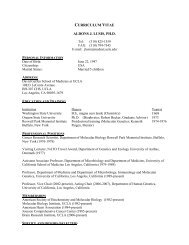
3 Relating modules to external clinical traits3.a Quantifying module–trait associationsIn this analysis we would like to identify modules that are significantly associated with the measured clinical traits.Since we already have a summary profile (eigengene) for each module, we simply correlate eigengenes with externaltraits and look for the most significant associations:# Define numbers of genes and samplesnGenes = ncol(datExpr);nSamples = nrow(datExpr);# Recalculate MEs with color labelsMEs0 = moduleEigengenes(datExpr, moduleColors)$eigengenesMEs = orderMEs(MEs0)moduleTraitCor = cor(MEs, datTraits, use = "p");moduleTraitPvalue = corPvalueStudent(moduleTraitCor, nSamples);Since we have a moderately large number of modules and traits, a suitable graphical representation will help inreading the table. We color code each association by the correlation value:sizeGrWindow(10,6)# Will display correlations and their p-valuestextMatrix = paste(signif(moduleTraitCor, 2), "\n(",signif(moduleTraitPvalue, 1), ")", sep = "");dim(textMatrix) = dim(moduleTraitCor)par(mar = c(6, 8.5, 3, 3));# Display the correlation values within a heatmap plotlabeledHeatmap(Matrix = moduleTraitCor,xLabels = names(datTraits),yLabels = names(MEs),ySymbols = names(MEs),colorLabels = FALSE,colors = greenWhiteRed(50),textMatrix = textMatrix,setStdMargins = FALSE,cex.text = 0.5,zlim = c(-1,1),main = paste("Module-trait relationships"))The resulting color-coded table is shown in Fig. 1.The analysis identifies the several significant module–trait associations. We will concentrate on weight as the traitof interest.3.b Gene relationship to trait and important modules: Gene Significance and ModuleMembershipWe quantify associations of individual genes with our trait of interest (weight) by defining Gene Significance GS as(the absolute value of) the correlation between the gene and the trait. For each module, we also define a quantitativemeasure of module membership MM as the correlation of the module eigengene and the gene expression profile. Thisallows us to quantify the similarity of all genes on the array to every module.# Define variable weight containing the weight column of datTraitweight = as.data.frame(datTraits$weight_g);names(weight) = "weight"# names (colors) of the modulesmodNames = substring(names(MEs), 3)geneModuleMembership = as.data.frame(cor(datExpr, MEs, use = "p"));MMPvalue = as.data.frame(corPvalueStudent(as.matrix(geneModuleMembership), nSamples));

MEmagentaMEblackMEturquoiseMEgreenMElightcyanMEgreenyellowMEblueMEbrownMEredMEsalmonMEyellowMElightgreenMEgreyMEpinkMEgrey60MEpurpleMEtanMEcyanMEmidnightblueweight_glength_cmab_fatother_fattotal_fatX100xfat_weightTriglyTotal_CholModule−trait relationships−0.017 0.08 −0.0056−0.033−0.017−0.0630.023 −0.037 0.053 −0.074 −0.13 −0.095−0.039−0.028−0.0110.082 −0.064 0.051 0.015−0.00110.19 −0.094−0.053−0.0340.08 0.015(0.8) (0.4) (0.9) (0.7) (0.8) (0.5) (0.8) (0.7) (0.5) (0.4) (0.1) (0.3) (0.7) (0.7) (0.9) (0.3) (0.5) (0.6) (0.9) (1) (0.03) (0.3) (0.5) (0.7) (0.4) (0.9)−0.31 −0.15 −0.27 −0.15 −0.24 −0.18 −0.073 −0.16 −0.07 −0.2 −0.24 −0.28 −0.15 0.055 −0.33 0.45 −0.37 −0.12 0.18 0.096 0.084 0.044 0.03 −0.044 −0.27 −0.29(2e−04) (0.07) (0.001) (0.09) (0.006) (0.04) (0.4) (0.07) (0.4) (0.02) (0.006)(9e−04)(0.08) (0.5) (1e−04)(7e−08)(1e−05)(0.2) (0.04) (0.3) (0.3) (0.6) (0.7) (0.6) (0.002)(6e−04)−0.27 −0.15 −0.33 −0.059 −0.24 −0.21 0.011 −0.094 −0.15 −0.063 0.029 −0.06 −0.088 0.02 −0.097 0.23 −0.38 −0.12 0.091 0.18 0.13 0.054 0.063 0.025 −0.25 −0.22(0.001) (0.09) (1e−04) (0.5) (0.005) (0.01) (0.9) (0.3) (0.09) (0.5) (0.7) (0.5) (0.3) (0.8) (0.3) (0.009)(4e−06)(0.2) (0.3) (0.04) (0.1) (0.5) (0.5) (0.8) (0.004) (0.01)0.0013 −0.13 −0.034 0.22 0.078 0.11 −0.1 0.036 −0.18 0.03 −0.013−0.0260.043 0.051 −0.051 0.15 −0.22 −0.1 0.17 0.22 0.16 0.074 0.043−0.0016−0.28−0.22(1) (0.1) (0.7) (0.01) (0.4) (0.2) (0.3) (0.7) (0.03) (0.7) (0.9) (0.8) (0.6) (0.6) (0.6) (0.09) (0.01) (0.2) (0.06) (0.01) (0.07) (0.4) (0.6) (1) (9e−04)(0.009)−0.13 −0.12 −0.2 0.076 −0.087−0.086−0.05 −0.1 −0.1 −0.11 −0.081 −0.16 −0.1 0.067 −0.12 0.25 −0.3 −0.12 0.18 0.21 0.2 0.033 0.12 0.059 −0.29 −0.27(0.1) (0.2) (0.02) (0.4) (0.3) (0.3) (0.6) (0.2) (0.2) (0.2) (0.4) (0.06) (0.3) (0.4) (0.2) (0.004)(5e−04)(0.2) (0.04) (0.02) (0.02) (0.7) (0.2) (0.5) (6e−04)(0.002)−0.022 0.05 0.024 0.13 0.087 0.13 −0.043−0.029−0.083−0.018−0.03 −0.076−0.026−0.0970.066 −0.14 −0.085 −0.12−0.00290.0930.049 −0.078 0.024 −0.061 0.078−0.0017(0.8) (0.6) (0.8) (0.1) (0.3) (0.1) (0.6) (0.7) (0.3) (0.8) (0.7) (0.4) (0.8) (0.3) (0.4) (0.1) (0.3) (0.2) (1) (0.3) (0.6) (0.4) (0.8) (0.5) (0.4) (1)0.31 0.036 0.29 0.23 0.29 0.26 −0.011 0.098 −0.086 0.068 0.065 0.15 0.1 0.24 0.02 −0.12 0.25 0.062 0.19 −0.086 −0.16 −0.087 −0.22 −0.18 −0.088−0.023(2e−04) (0.7) (6e−04)(0.008)(7e−04)(0.002)(0.9) (0.3) (0.3) (0.4) (0.5) (0.07) (0.2) (0.006) (0.8) (0.2) (0.003) (0.5) (0.03) (0.3) (0.06) (0.3) (0.01) (0.04) (0.3) (0.8)0.59 0.1 0.48 0.47 0.53 0.51 −0.15 0.33 0.075 0.33 0.32 0.34 0.32 0.13 0.34 −0.43 0.43 0.069 −0.11 −0.082 −0.12 0.071 −0.0980.0093−0.0320.068(5e−14) (0.2) (3e−09)(9e−09)(3e−11)(3e−10)(0.09) (1e−04) (0.4) (8e−05)(1e−04)(6e−05)(1e−04)(0.1) (5e−05)(3e−07)(2e−07)(0.4) (0.2) (0.3) (0.2) (0.4) (0.3) (0.9) (0.7) (0.4)0.51 0.15 0.42 0.43 0.47 0.45 0.035 0.34 0.1 0.28 0.2 0.29 0.34 0.096 0.27 −0.41 0.42 0.13 −0.1 −0.16 −0.11 −0.092 −0.14 −0.029 0.07 0.12(3e−10) (0.08) (6e−07)(3e−07)(1e−08)(6e−08)(0.7) (6e−05) (0.2) (0.001) (0.02) (8e−04)(7e−05)(0.3) (0.002)(1e−06)(4e−07)(0.1) (0.2) (0.07) (0.2) (0.3) (0.1) (0.7) (0.4) (0.2)0.43 0.22 0.36 0.3 0.37 0.32 0.17 0.27 0.13 0.29 0.35 0.33 0.26 −0.11 0.47 −0.58 0.26 −0.011 −0.12 −0.081−0.0610.15 0.032 0.13 0.13 0.17(2e−07) (0.01) (2e−05)(5e−04)(8e−06)(1e−04)(0.06) (0.002) (0.1) (6e−04)(3e−05)(9e−05)(0.002)(0.2) (1e−08)(3e−13)(0.002)(0.9) (0.2) (0.4) (0.5) (0.09) (0.7) (0.1) (0.1) (0.05)0.22 0.05 0.18 0.22 0.21 0.2 0.1 0.3 0.075 0.37 0.42 0.41 0.3 −0.16 0.41 −0.46 0.2 0.013 −0.11−0.0026−0.0460.13 0.03 0.085 0.22 0.33(0.01) (0.6) (0.04) (0.01) (0.01) (0.02) (0.2) (4e−04) (0.4) (1e−05)(4e−07)(6e−07)(5e−04)(0.06) (7e−07)(2e−08)(0.02) (0.9) (0.2) (1) (0.6) (0.1) (0.7) (0.3) (0.01) (1e−04)−0.057 0.13 −0.0094−0.047−0.03 −0.015 0.01 −0.031 0.067 −0.047−0.055−0.018−0.033−0.062−0.0210.069 −0.15 −0.024 0.065 0.011 0.04 0.048 0.00044 0.031 0.14 0.099(0.5) (0.1) (0.9) (0.6) (0.7) (0.9) (0.9) (0.7) (0.4) (0.6) (0.5) (0.8) (0.7) (0.5) (0.8) (0.4) (0.07) (0.8) (0.5) (0.9) (0.6) (0.6) (1) (0.7) (0.1) (0.3)0.09 0.14 0.15 −0.015 0.11 0.09 −0.05−0.00380.13 −0.0099−0.0052−0.047−0.0084−0.21−0.037−0.0250.061 −0.058 −0.02 −0.028−0.0260.15 −0.054 0.08 0.079 0.069(0.3) (0.1) (0.09) (0.9) (0.2) (0.3) (0.6) (1) (0.1) (0.9) (1) (0.6) (0.9) (0.02) (0.7) (0.8) (0.5) (0.5) (0.8) (0.7) (0.8) (0.09) (0.5) (0.4) (0.4) (0.4)−0.051 0.072 0.013 −0.24 −0.1 −0.13 0.052 −0.15 0.067 −0.21 −0.26 −0.23 −0.15 0.045 −0.17 0.1 0.16 0.11 −0.064 −0.17 −0.096 −0.17 −0.091−0.0620.16 0.04(0.6) (0.4) (0.9) (0.005) (0.2) (0.1) (0.5) (0.08) (0.4) (0.02) (0.002)(0.008)(0.07) (0.6) (0.06) (0.2) (0.06) (0.2) (0.5) (0.05) (0.3) (0.04) (0.3) (0.5) (0.07) (0.6)−0.017−0.0730.061 0.0097 0.045 0.077 −0.021 0.025 0.0029 0.067 0.061 0.046 0.024 0.029 −0.087 0.19 0.0069 0.12 −0.016−0.062−0.062−0.0047−0.099−0.054−0.03 −0.085(0.8) (0.4) (0.5) (0.9) (0.6) (0.4) (0.8) (0.8) (1) (0.4) (0.5) (0.6) (0.8) (0.7) (0.3) (0.03) (0.9) (0.2) (0.9) (0.5) (0.5) (1) (0.3) (0.5) (0.7) (0.3)−0.021−0.0220.049 −0.096−0.0120.0054−0.0068−0.079−0.092−0.092−0.15 −0.091−0.076−0.098−0.075−0.0340.096 0.061 0.042 0.0018 −0.07 −0.099 0.018 −0.1 0.076 0.049(0.8) (0.8) (0.6) (0.3) (0.9) (1) (0.9) (0.4) (0.3) (0.3) (0.08) (0.3) (0.4) (0.3) (0.4) (0.7) (0.3) (0.5) (0.6) (1) (0.4) (0.3) (0.8) (0.2) (0.4) (0.6)0.27 0.18 0.32 0.15 0.28 0.27 −0.014 0.21 0.16 0.21 0.14 0.23 0.21 −0.11 0.2 −0.32 0.28 0.034 −0.12 −0.12 −0.098 0.11 −0.018−0.00880.26 0.32(0.002) (0.04) (2e−04) (0.08) (0.001)(0.002)(0.9) (0.01) (0.06) (0.02) (0.1) (0.007) (0.02) (0.2) (0.02) (2e−04)(8e−04)(0.7) (0.2) (0.2) (0.3) (0.2) (0.8) (0.9) (0.002)(2e−04)0.18 0.15 0.25 0.061 0.18 0.15 −0.075 0.044 0.2 −0.0037−0.12−0.065 0.037 −0.022 0.014 −0.12 0.22 0.047 −0.08 −0.16 −0.052 0.084 −0.03 0.058 0.076 0.016(0.04) (0.07) (0.004) (0.5) (0.03) (0.09) (0.4) (0.6) (0.02) (1) (0.2) (0.5) (0.7) (0.8) (0.9) (0.2) (0.01) (0.6) (0.4) (0.06) (0.5) (0.3) (0.7) (0.5) (0.4) (0.9)0.19 −0.024 0.22 0.27 0.27 0.28 −0.11 0.13 −0.052 0.11 0.0012 0.031 0.13 0.015 0.011 −0.04 0.035 −0.02 0.075 0.065 0.047 0.15 −0.0190.0039−0.12 −0.076(0.03) (0.8) (0.01) (0.002) (0.002)(9e−04)(0.2) (0.1) (0.5) (0.2) (1) (0.7) (0.1) (0.9) (0.9) (0.6) (0.7) (0.8) (0.4) (0.5) (0.6) (0.08) (0.8) (1) (0.2) (0.4)HDL_CholUCFFAGlucoseLDL_plus_VLDLMCP_1_physInsulin_ug_lGlucose_InsulinLeptin_pg_mlAdiponectinAortic.lesionsAneurysmAortic_cal_MAortic_cal_LCoronaryArtery_CalMyocardial_calBMD_all_limbsBMD_femurs_only1.00.50.0−0.5−1.0Figure 1: Module-trait associations. Each row corresponds to a module eigengene, column to a trait. Each cellcontains the corresponding correlation and p-value. The table is color-coded by correlation according to the colorlegend.names(geneModuleMembership) = paste("MM", modNames, sep="");names(MMPvalue) = paste("p.MM", modNames, sep="");geneTraitSignificance = as.data.frame(cor(datExpr, weight, use = "p"));GSPvalue = as.data.frame(corPvalueStudent(as.matrix(geneTraitSignificance), nSamples));names(geneTraitSignificance) = paste("GS.", names(weight), sep="");names(GSPvalue) = paste("p.GS.", names(weight), sep="");3.c Intramodular analysis: identifying genes with high GS and MMUsing the GS and MM measures, we can identify genes that have a high significance for weight as well as high modulemembership in interesting modules. As an example, we look at the brown module that has the highest associationwith weight. We plot a scatterplot of Gene Significance vs. Module Membership in the brown module:module = "brown"column = match(module, modNames);moduleGenes = moduleColors==module;sizeGrWindow(7, 7);par(mfrow = c(1,1));verboseScatterplot(abs(geneModuleMembership[moduleGenes, column]),

abs(geneTraitSignificance[moduleGenes, 1]),xlab = paste("Module Membership in", module, "module"),ylab = "Gene significance for body weight",main = paste("Module membership vs. gene significance\n"),cex.main = 1.2, cex.lab = 1.2, cex.axis = 1.2, col = module)The plot is shown in Fig. 2. Clearly, GS and MM are highly correlated, illustrating that genes highly significantlyassociated with a trait are often also the most important (central) elements of modules associated with the trait.The reader is encouraged to try this code with other significance trait/module correlation (for example, the magenta,midnightblue, and red modules with weight).Module membership vs. gene significancecor=0.48 p=

will return probe IDs belonging to the brown module. To facilitate interpretation of the results, we use a probeannotation file provided by the manufacturer of the expression arrays to connect probe IDs to gene names anduniversally recognized identification numbers (Entrez codes).annot = read.csv(file = "GeneAnnotation.csv");dim(annot)names(annot)probes = names(datExpr)probes2annot = match(probes, annot$substanceBXH)# The following is the number or probes without annotation:sum(is.na(probes2annot))# Should return 0.We now create a data frame holding the following information for all probes: probe ID, gene symbol, Locus Link ID(Entrez code), module color, gene significance for weight, and module membership and p-values in all modules. Themodules will be ordered by their significance for weight, with the most significant ones to the left.# Create the starting data framegeneInfo0 = data.frame(substanceBXH = probes,geneSymbol = annot$gene_symbol[probes2annot],LocusLinkID = annot$LocusLinkID[probes2annot],moduleColor = moduleColors,geneTraitSignificance,GSPvalue)# Order modules by their significance for weightmodOrder = order(-abs(cor(MEs, weight, use = "p")));# Add module membership information in the chosen orderfor (mod in 1:ncol(geneModuleMembership)){oldNames = names(geneInfo0)geneInfo0 = data.frame(geneInfo0, geneModuleMembership[, modOrder[mod]],MMPvalue[, modOrder[mod]]);names(geneInfo0) = c(oldNames, paste("MM.", modNames[modOrder[mod]], sep=""),paste("p.MM.", modNames[modOrder[mod]], sep=""))}# Order the genes in the geneInfo variable first by module color, then by geneTraitSignificancegeneOrder = order(geneInfo0$moduleColor, -abs(geneInfo0$GS.weight));geneInfo = geneInfo0[geneOrder, ]This data frame can be written into a text-format spreadsheet, for example bywrite.csv(geneInfo, file = "geneInfo.csv")The reader is encouraged to open and view the file in a spreadsheet software, or inspect it directly within R usingthe command fix(geneInfo).