Function Approximation Using Artificial Neural Networks
Function Approximation Using Artificial Neural Networks
Function Approximation Using Artificial Neural Networks

You also want an ePaper? Increase the reach of your titles
YUMPU automatically turns print PDFs into web optimized ePapers that Google loves.
INTERNATIONAL JOURNAL OF SYSTEMS APPLICATIONS, ENGINEERING & DEVELOPMENT Issue 4, Volume 1, 2007<br />
<strong>Function</strong> <strong>Approximation</strong> <strong>Using</strong> <strong>Artificial</strong> <strong>Neural</strong> <strong>Networks</strong><br />
ZARITA ZAINUDDIN & ONG PAULINE<br />
School of Mathematical Sciences<br />
Universiti Sains Malaysia<br />
11800 Minden, Penang<br />
MALAYSIA<br />
zarita@cs.usm.my<br />
Abstract: - <strong>Function</strong> approximation, which finds the underlying relationship from a given finite input-output<br />
data is the fundamental problem in a vast majority of real world applications, such as prediction, pattern<br />
recognition, data mining and classification. Various methods have been developed to address this problem,<br />
where one of them is by using artificial neural networks. In this paper, the radial basis function network and<br />
the wavelet neural network are applied in estimating periodic, exponential and piecewise continuous functions.<br />
Different types of basis functions are used as the activation function in the hidden nodes of the radial basis<br />
function network and the wavelet neural network. The performance is compared by using the normalized<br />
square root mean square error function as the indicator of the accuracy of these neural network models.<br />
Key-Words: - function approximation, artificial neural network, radial basis function network, wavelet neural<br />
network<br />
1 Introduction<br />
Learning a mapping between an input and an output<br />
space from a set of input-output data is the core<br />
concern in diverse real world applications. Instead<br />
of an explicit formula to denote the function f, only<br />
pairs of input-output data in the form of (x, f(x)) are<br />
available.<br />
m<br />
Let x ∈ R ,<br />
i<br />
i = 1,2,…,N<br />
1<br />
d i<br />
∈ R , i = 1,2,…,N<br />
be the N input vectors with dimension m and N real<br />
number output respectively. We seek an unknown<br />
function f(x):R m →R 1 that satisfies the interpolation<br />
where<br />
f (x i ) = d i , i = 1,2,…,N (2)<br />
The goodness of fit of d i by the function f, is<br />
given by an error function. A commonly used error<br />
function is defined by<br />
E(<br />
f ) =<br />
1<br />
2<br />
N<br />
∑<br />
i=<br />
1<br />
N<br />
( d i<br />
− y i<br />
)<br />
1<br />
2<br />
= ∑[(<br />
di − f ( x i<br />
))]<br />
2 i=<br />
1<br />
where y i is the actual response.<br />
In short, the main concern is to minimize the<br />
error function. In the other words, to enhance the<br />
accuracy of the estimation is the principal objective<br />
of function approximation.<br />
There exist multiple methods that have been<br />
established as function approximation tools, where<br />
an artificial neural network (ANNs) is one of them.<br />
2<br />
(1)<br />
(3)<br />
According to Cybenko [1] and Hornik [2], there<br />
exists a three layer neural network that is capable in<br />
estimating an arbitrary nonlinear function f with any<br />
desired accuracy. Hence, it is not surprising that<br />
ANNs have been employed in various applications,<br />
especially in issues related to function<br />
approximation, due to its capability in finding the<br />
pattern within input-output data without the need for<br />
predetermined models. Among all the models of<br />
ANNs, the multilayer perceptron (MLP) is the most<br />
commonly used.<br />
Nevertheless, MLP itself has certain<br />
shortcomings. Firstly, MLP tends to get trapped in<br />
undesirable local minima in order to reach the global<br />
minimum of a very complex search space. Secondly,<br />
training of MLP is highly time consuming, due to<br />
the slow converging of MLP. Thirdly, MLP also<br />
fails to converge when high nonlinearities exist.<br />
Thus, these drawbacks deteriorate the accuracy of<br />
the MLP in function approximation [3, 4, 5].<br />
To overcome the obstacles encountered by using<br />
an MLP, a radial basis function network (RBFN),<br />
which has been introduced by replacing the global<br />
activation function in MLP with a localized radial<br />
basis function, has been found to perform better than<br />
the MLP in function approximation [6,7].<br />
The idea of combining wavelet basis functions<br />
and a three layer neural network has resulted in the<br />
wavelet neural network (WNN), which has a similar<br />
architecture with the RBFN. Since the first<br />
implementation of the WNN by Zhang and<br />
Benveniste [8, 9, 10], it has received tremendous<br />
173 Manuscript Received June 14, 2007; Revised December 24, 2007
INTERNATIONAL JOURNAL OF SYSTEMS APPLICATIONS, ENGINEERING & DEVELOPMENT Issue 4, Volume 1, 2007<br />
attention from other researchers [11, 12, 13, 14] due<br />
its great improvement over the weaknesses of MLP.<br />
This paper is organized as follows. In sections 2<br />
and 3, a brief introduction of RBFN and WNN is<br />
presented. The types of basis functions used in this<br />
paper are given in section 4, while numerical<br />
simulations of both neural network models in<br />
function approximation are discussed in section 5,<br />
where the performance of RBFN and WNN are<br />
compared in terms of the normalized square root<br />
mean square error function. Lastly, conclusions are<br />
drawn in section 6.<br />
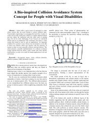
2 Radial Basis <strong>Function</strong> Network<br />
Radial basis function network was first introduced<br />
by Broomhead and Lowe in 1988 [6], which is just<br />
the association of radial functions into a single<br />
hidden layer neural network, such as shown in<br />
Figure 1.<br />
w 1<br />
φ 1<br />
x 1<br />
φ 2<br />
. . . . . .<br />
. . . . . . . . .<br />
Figure 1: Radial basis function network<br />
A RBFN is a standard three layer neural network,<br />
with the first input layer consisting of of d input<br />
nodes, one hidden layer consisting of m radial basis<br />
functions in the hidden nodes and a linear output<br />
layer. There is an activation function φ for each of<br />
the hidden node. Each of the hidden node receives<br />
<br />
multiple inputs x = ( x 1<br />
,..., x d<br />
) and produces one<br />
output y. It is determined by a center c and a<br />
parameter b which is called the width, where<br />
<br />
φ<br />
j<br />
( ξ ) = φ<br />
j<br />
( x − c / b),<br />
j = 1,...,<br />
m . (4)<br />
φ can be any suitable radial basis function, such as<br />
Gaussian, Multiquadrics and Inverse Multiquadrics.<br />
Thus, the RBFN output is given by<br />
y =<br />
y<br />
Σ<br />
m<br />
w j<br />
j=<br />
1<br />
∑<br />
φ ( ξ )<br />
j<br />
x d<br />
w m<br />
φ m<br />
Output<br />
Layer<br />
Hidden<br />
Layer<br />
Input<br />
Layer<br />
(5)<br />
where φ<br />
j<br />
( x)<br />
is the response of the jth hidden node<br />
resulting from all input data, w<br />
j<br />
is the connecting<br />
weight between the jth hidden node and output<br />
node, and m is the number of hidden nodes. The<br />
center vectors, c , the output weights w j and the<br />
width parameter b are adjusted adaptively during the<br />
training of RBFN in order to fit the data well.<br />
2.1 Learning of Radial Basis <strong>Function</strong><br />
Network<br />
By means of learning, RBFN tends to find the<br />
network parameters c<br />
i<br />
,b and w i<br />
, such that the<br />
network output y ( x i<br />
) fits the unknown underlying<br />
function f ( x i<br />
) of a certain mapping between the<br />
input-output data as close as possible. This is done<br />
by minimizing an error function, such as in Equation<br />
3.<br />
The learning in RBFN is done in two stages.<br />
Firstly, the widths and the centers are fixed. Next,<br />
the weights are found by solving the linear equation.<br />
There are a few ways to select the parameter centers,<br />
c<br />
i<br />
. It can be randomly chosen from input data, or<br />
from the cluster means. The parameter width, b,<br />
usually is fixed. Once the centers have been<br />
selected, the weights that minimize the output error<br />
are computed by solving a linear pseudoinverse<br />
solution.<br />
Let us represent the network output for all input<br />
data, d, in Equation (5) as Y = Φ W where<br />
⎛ϕ(<br />
x1,<br />
c1<br />
) ϕ(<br />
x1,<br />
c2)<br />
... ϕ(<br />
x1,<br />
cm)<br />
⎞<br />
⎜<br />
⎟<br />
⎜ϕ(<br />
x2,<br />
c1<br />
) ϕ(<br />
x2,<br />
c2)<br />
... ϕ(<br />
x2,<br />
cm)<br />
⎟<br />
Φ = ⎜ : : : : ⎟ (6)<br />
⎜<br />
⎟<br />
⎝ϕ(<br />
xd<br />
, c1<br />
) ϕ(<br />
xd<br />
, c2)<br />
... ϕ(<br />
xd<br />
, cm)<br />
⎠<br />
is the output of basis functions ϕ , and<br />
(7)<br />
ϕ x , c ) = ϕ(||<br />
x − c ||)<br />
(<br />
i j<br />
i j<br />
Hence, the weight matrix W can be solved as<br />
W = Φ + Y<br />
where Φ + is the pseudoinverse defined as<br />
Φ + = (Φ T Φ) -1 Φ T<br />
3 Wavelet <strong>Neural</strong> Network<br />
By incorporating the time-frequency localization<br />
properties of wavelet basis functions and the<br />
learning abilities of ANN, WNN has yet become<br />
another suitable tool in function approximation [8, 9,<br />
10, 14].<br />
WNN shares a similar network architecture as<br />
RBFN [15, 16], such as shown in Figure 1. Instead<br />
(8)<br />
(9)<br />
174
INTERNATIONAL JOURNAL OF SYSTEMS APPLICATIONS, ENGINEERING & DEVELOPMENT Issue 4, Volume 1, 2007<br />
of the radial basis function, wavelet frames such as<br />
Gaussian wavelet, Morlet and Mexican Hat are used<br />
as the activation functions in the hidden nodes,<br />
while the center vectors and parameters of width in<br />
RBFN are replaced by translation E and dilation<br />
vectors T<br />
j<br />
respectively. In fact, RBFN and WNN<br />
have been proven that they are actually specific<br />
cases of a generic paradigm, called Weighted Radial<br />
Basis <strong>Function</strong>s [15].<br />
Similar to RBFN, WNN has a model based on<br />
Euclidean distance between the input vector x and<br />
translation vector E j<br />
, where each of the distance<br />
components is weighted by a dilation vector T j<br />
.<br />
Thus, the output of WNN is given by<br />
M<br />
X − E j<br />
y = ∑Φ<br />
j<br />
( )<br />
(6)<br />
j = 1 T j<br />
where M is the number of hidden nodes.<br />
Learning of WNN is similar to that of RBFN as<br />
discussed in section 2.1, where the parameters of the<br />
center and width of radial basis function in RBFN<br />
are replaced by the parameters of translation and<br />
dilation of the wavelet basis function in WNN<br />
respectively.<br />
4 Types of Basis <strong>Function</strong><br />
In fact, RBFN and WNN are very similar to each<br />
other. The difference lies in the types of activation<br />
functions used in the hidden nodes of the hidden<br />
layer. Different types of basis functions that are used<br />
in this paper are given below (see Fig. 2):<br />
i. Mexican Hat<br />
⎛ X E ⎞<br />
2<br />
( z)<br />
⎜ −<br />
Φ = Φ ⎟ = ( n − 2z<br />
).exp( −z<br />
⎜ T ⎟<br />
⎝ ⎠<br />
where n = dim(z)<br />
ii.<br />
iii.<br />
iv.<br />
Gaussian Wavelet<br />
⎛ X E ⎞<br />
2<br />
( z)<br />
⎜ −<br />
Φ = Φ ⎟ = ( −z).exp(<br />
−z<br />
⎜ T ⎟<br />
⎝ ⎠<br />
Mexican Hat<br />
⎛ X E ⎞<br />
2<br />
( z)<br />
⎜ −<br />
Φ = Φ ⎟ = cos(5z).exp(<br />
−z<br />
⎜ T ⎟<br />
⎝ ⎠<br />
Gaussian<br />
2<br />
G(<br />
z)<br />
= G(||<br />
x − ci ||) = exp( −z<br />
)<br />
where i = 1,2,...,<br />
N<br />
j<br />
2<br />
);<br />
/ 2)<br />
/ 2)<br />
(9)<br />
(10)<br />
(7)<br />
(8)<br />
(a) Mexican Hat<br />
(c) Morlet<br />
(d) Gaussian<br />
Figure 2: Types of basis functions<br />
5 Numerical Simulations<br />
In this section, we present experimental results of<br />
RBFN and WNN in approximating different types of<br />
functions. It includes a continuous function with one<br />
and two variables, and also a piecewise continuous<br />
function with one variable. Different types of basis<br />
functions will be used as the activation function in<br />
the hidden nodes of RBFN and WNN, namely, the<br />
Gaussian, Gaussian Wavelet, Morlet and Mexican<br />
Hat. The simulation is done by using Matlab<br />
Version 7.0 [17].<br />
To evaluate the approximation results, an error<br />
criterion is needed. The normalized square root<br />
mean square error function (N e ) is chosen as the<br />
error criterion, that is,<br />
nt<br />
1<br />
( i)<br />
( i)<br />
2<br />
Ne<br />
= ∑(<br />
y − f )<br />
(11)<br />
σ<br />
y<br />
i=<br />
1<br />
(b) Gaussian Wavelet<br />
where f (i) and y (i) are the output of network and<br />
desirable value of the function to be approximated ,<br />
nt is the total number of testing samples and σ<br />
y<br />
is<br />
the standard deviation of the output value. A smaller<br />
N e indicates higher accuracy.<br />
For function approximation of continuous<br />
functions with one variable, as in Case 1 and Case<br />
2, these functions were sampled at 100 uniformly<br />
spaced training points in the domain [-1,1], while<br />
the testing samples consists of 200 points, which<br />
were also sampled uniformly in the same domain.<br />
For the continuous functions with two variables,<br />
as in Case 3 and Case 4, 200 training points and 350<br />
testing points in the domain [-1,1] were used.<br />
175
INTERNATIONAL JOURNAL OF SYSTEMS APPLICATIONS, ENGINEERING & DEVELOPMENT Issue 4, Volume 1, 2007<br />
Lastly, for the piecewise continuous function as<br />
in Case 5, we sample the function to yield 200<br />
points distributed uniformly over [-10, 10] as<br />
training data. For testing data, 200 points which<br />
were uniformly sampled over [-10, 10] were used.<br />
5.1 Case 1: 1-D Continuous Exponential<br />
<strong>Function</strong><br />
y = ( x + 1)exp( −3x<br />
+ 3)<br />
(12)<br />
The simulation result for Case 1 by using RBFN and<br />
WNN with different basis functions is shown in<br />
Table 1, in terms of N e . Fig. 3 shows the results for<br />
the approximation of the function in Case 1.<br />
5.2 Case 2: 1-D Continuous Periodic<br />
<strong>Function</strong><br />
y = sin( 4π<br />
x)exp(<br />
− | 5x<br />
|)<br />
The simulation result for Case 2 by using RBFN and<br />
WNN with different basis functions is shown in<br />
Table 2, in terms of N e . Fig. 4 shows the results for<br />
the approximation of the function in Case 2.<br />
Table 2: Simulation Result for Case 2<br />
Model Basis <strong>Function</strong> N e<br />
RBFN Gaussian 9.11658<br />
WNN Gaussian Wavelet 0.207205<br />
Mexican Hat 6.09464<br />
Morlet 3.98573<br />
(13)<br />
Table 1: Simulation Result for Case 1<br />
Model Basis <strong>Function</strong> N e<br />
RBFN Gaussian 2.64481e-005<br />
WNN Gaussian Wavelet 0.0210695<br />
Mexican Hat 9.41899e-005<br />
Morlet<br />
4.11055e-005<br />
0.6<br />
0.4<br />
0.2<br />
0<br />
-0.2<br />
Exact<br />
Gaussian<br />
Gaussian Wavelet<br />
Mexican Hat<br />
Morlet<br />
4.5<br />
Exact<br />
Gaussian<br />
Gaussian Wavelet<br />
Mexican Hat<br />
Morlet<br />
-0.4<br />
-0.6<br />
-0.8<br />
-1 -0.8 -0.6 -0.4 -0.2 0 0.2 0.4 0.6 0.8 1<br />
4<br />
Figure 4: Simulation result for Case 2<br />
3.5<br />
0.68 0.685 0.69 0.695 0.7 0.705 0.71 0.715 0.72 0.725 0.73<br />
Figure 3: Simulation result for Case 1-zoom in<br />
From Table 1, RBFN with Gaussian as the basis<br />
function gives the best performance. It is stated in<br />
[16] that RBFN approximates an exponential<br />
function well. Hence, in Case 1 where a 1-D<br />
exponential function is used, RBFN outperforms<br />
WNN. The wavelet basis functions used have the<br />
same characteristics, namely, they are crude,<br />
symmetric and irregular in shape, compactly<br />
supported, which means they vanish outside a finite<br />
interval and have explicit expression. However,<br />
among all the wavelet basis functions used,<br />
Gaussian wavelet yields the lowest accuracy. It is<br />
probably due to the shape of Gaussian wavelet,<br />
which is less similar to the function used in Case 1.<br />
Hence, it could not adapt well to the shape of this<br />
exponential function.<br />
From Table 2, WNN with Gaussian wavelet as the<br />
basis function gives the best performance. In Case 2<br />
a 1-D periodic function is used. A periodic function<br />
is approximated better by WNN with an oscillating<br />
wavelet basis function [16]. Hence, it is shown in<br />
Table 2 that RBFN gives the lowest accuracy.<br />
Among all the wavelet basis functions, Gaussian<br />
wavelet performs the best. The good performance of<br />
Gaussian wavelet, as demonstrated in Fig. 4, is<br />
probably due to its similar shape with the function<br />
used in Case 2.<br />
5.3 Case 3: 2-D Continuous Exponential<br />
<strong>Function</strong><br />
z = 2sin(π e -x2-y2 )<br />
(14)<br />
The simulation result for Case 3 by using RBFN and<br />
WNN with different basis functions is shown in<br />
Table 3, in terms of N e .<br />
176
INTERNATIONAL JOURNAL OF SYSTEMS APPLICATIONS, ENGINEERING & DEVELOPMENT Issue 4, Volume 1, 2007<br />
Table 3: Simulation Result for Case 3<br />
Model Basis <strong>Function</strong> N e<br />
RBFN Gaussian 0.117956<br />
WNN Gaussian Wavelet 0.194523<br />
Mexican Hat 0.17059<br />
Morlet 0.15684<br />
Table 5: Simulation Result for Case 5<br />
Model Basis <strong>Function</strong> N e<br />
RBFN Gaussian 0.899789<br />
WNN Gaussian Wavelet 2.71425e-013<br />
Mexican Hat 0.752215<br />
Morlet 0.650081<br />
From Table 3, it can be observed that the accuracy<br />
of WNN with different types of basis function are<br />
comparatively close to each other. However, RBFN<br />
outperforms WNN since the function used in Case 3<br />
is an exponential function.<br />
Target Vector y<br />
1.5<br />
1<br />
0.5<br />
0<br />
Exact<br />
Gaussian<br />
Mexican Hat<br />
Morlet<br />
Gaussian Wavelet<br />
5.4 Case 4: 2-D Continuous Periodic<br />
<strong>Function</strong><br />
z = 2(1-x 2 -y 2 )e -x2-y2 + sin[(x 2 +y 2 )e -(x2-y2)/2 ]<br />
(14)<br />
-0.5<br />
-1<br />
-1 -0.8 -0.6 -0.4 -0.2 0 0.2 0.4 0.6 0.8 1<br />
Input Vector x<br />
Figure 5: Simulation result for Case 5<br />
The simulation result for Case 4 by using RBFN and<br />
WNN with different basis functions is shown in<br />
Table 4, in terms of N e .<br />
-0.6<br />
-0.65<br />
-0.7<br />
Exact<br />
Gaussian<br />
Mexican Hat<br />
Morlet<br />
Gaussian Wavelet<br />
Table 4: Simulation Result for Case 4<br />
Model Basis <strong>Function</strong> N e<br />
RBFN Gaussian 0.26292<br />
WNN Gaussian Wavelet 0.254194<br />
Mexican Hat 0.174942<br />
Morlet 0.114205<br />
It is shown in Table 4 that WNN with Morlet as the<br />
basis function performs the best in comparison to<br />
the others. It could probably due to the shape of<br />
Morlet which is more identical to the shape of the<br />
function in Case 4. WNN outperforms RBFN in<br />
estimating a periodic function due to the oscillating<br />
behavior of the wavelet basis function which can<br />
capture the characteristic of a periodic function well.<br />
Hence, RBFN gives the highest error in Case 4.<br />
5.5 Case 5: Piecewise Continuous <strong>Function</strong><br />
A piecewise continuous function<br />
⎧<br />
⎪<br />
f ( x)<br />
⎨<br />
⎪<br />
⎩10e<br />
−2.186x<br />
−12.864<br />
−0.05x−0.5<br />
4.264x<br />
sin[(0.03x<br />
+ 0.7) x]<br />
−10≤<br />
x < −2<br />
−2<br />
≤ x < 0<br />
0 ≤ x ≤10<br />
(15)<br />
is used in this case. Simulation result in terms of N e<br />
is shown in Table 5 while the results of<br />
approximation of the piecewise continuous function<br />
above are given in Figs. 5 and 6.<br />
Target Vector y<br />
-0.75<br />
-0.8<br />
-0.85<br />
-0.9<br />
-0.95<br />
-0.3 -0.25 -0.2 -0.15 -0.1 -0.05<br />
Input Vector x<br />
Figure 6: Simulation result for Case 5-zoom in<br />
The function used in Case 5 is a piecewise<br />
continuous function, with a sharp spike at the<br />
interval (-0.3,-0.1). It is shown in Table 5 that WNN<br />
outperforms RBFN, especially in approximating the<br />
sharp spike, as shown in Figure 6. It is due to the<br />
irregular shape and fast oscillating characteristics of<br />
the wavelet functions, which leads them to<br />
approximate a function with sharp changes<br />
efficiently. Among all the wavelet basis functions,<br />
Gaussian wavelet gives the best performance. It is<br />
probably due to the shape of the Gaussian wavelet<br />
which is more identical to the piecewise function<br />
used in Case 5.<br />
5.6 Discussion<br />
An exponential function and a periodic function are<br />
approximated more accurately with RBFN and<br />
WNN respectively. It is mainly due to the basis<br />
functions that are used in the hidden nodes. WNN<br />
with an “oscillating” wavelet function tends to<br />
capture the behavior of a periodic function better<br />
177
INTERNATIONAL JOURNAL OF SYSTEMS APPLICATIONS, ENGINEERING & DEVELOPMENT Issue 4, Volume 1, 2007<br />
due to its oscillating characteristic. Hence, in Case 2<br />
and Case 4 which involve the approximation of a<br />
periodic function, it is observed that wavelet basis<br />
function outperforms radial basis function in terms<br />
of accuracy. However, in Case 1 and Case 3, where<br />
an exponential function is used, the accuracy of<br />
WNN and RBN is vice versa.<br />
The function used in Case 5 is a piecewise<br />
continuous function. From the simulation result, it is<br />
observed that WNN shows a higher accuracy than<br />
RBFN, especially in approximating the sharp spike,<br />
which is shown in Figure 6. It is due to the irregular<br />
shape of the wavelet functions, which leads them to<br />
analyze function with discontinuity or sharp changes<br />
efficiently.<br />
The wavelet basis functions used in this paper<br />
have the same characteristics, where they are crude,<br />
symmetric and have explicit expression.<br />
6 Conclusion<br />
This paper presents function approximation by using<br />
radial basis function network and wavelet neural<br />
network. WNN performs better in approximating a<br />
periodic function, whereas RBFN yields higher<br />
accuracy in estimating exponential function. In<br />
capturing the sharp spike in a piecewise function,<br />
WNN outshines RBFN due to its intrinsic<br />
characteristic.<br />
References:<br />
[1] Cybenko, G., <strong>Approximation</strong> by Superposition<br />
of a Sigmoidal <strong>Function</strong>, Mathematics Control<br />
Signals Systems, Vol. 2, 1989, pg 303-314.<br />
[2] Hornik, K., M. Stinchcombe & H. White,<br />
Multilayer Feedforward <strong>Networks</strong> are Universal<br />
Approximator, <strong>Neural</strong> <strong>Networks</strong>, Vol. 2, 1989,<br />
pg 359-3661.<br />
[3] M.H. Ahmad Fadzil & Zarita Zainuddin,<br />
Optimization of Learning Methods for Face<br />
Recognition using Multilayer Perceptron,<br />
Proceedings of the 3 rd IASTED Int. Conf. On<br />
Signal and Image Processing, Honolulu, Hawaii,<br />
USA, Aug 13-16 2001.<br />
[4] Zarita Zainuddin & Evans, D.J., “Human Face<br />
Recognition using Accelerated Multilayer<br />
Perceptrons”, International Journal of Computer<br />
Mathematics, Vol. 80, No.5, pg 535-558<br />
[5] Haykin,S., <strong>Neural</strong> Network: A Comprehensive<br />
Foundation, New York: Mc Millan Publishing<br />
Company, 1994<br />
[6] Broomhead, D.S., Lowe, D,. Multivariable<br />
function interpolation and adaptive networks.<br />
Complex Systems , Vol. 2, 1988, pg 321-335.<br />
[7] J.Moody, C. Darken, Learning with localized<br />
receptive fields, in: D.Touretzky, G.Hinton,<br />
T.Sejnowski (Eds), Proceedings of the 1988<br />
Connectionist Models Summer School, San<br />
Mateo, CA, 1989<br />
[8] Q. Zhang, <strong>Using</strong> Wavelet Network in<br />
Nonparametric Estimation, IEEE Transactions<br />
on <strong>Neural</strong> <strong>Networks</strong>, Vol.8, No.2, 1997, pg227-<br />
236<br />
[9] Q.Zhang, A. Benveniste, Wavelet <strong>Networks</strong>,<br />
IEEE Transactions on <strong>Neural</strong> <strong>Networks</strong>, Vol 3,<br />
No. 6, 1992, pg889-898<br />
[10] Q.Zhang, A. Benveniste, “<strong>Approximation</strong> by<br />
Nonlinear Wavelet <strong>Networks</strong>”, IEEE<br />
Transactions on <strong>Neural</strong> <strong>Networks</strong>, Vol 6, No. 10,<br />
1991, pg 3417-3420.<br />
[11] A. Subasi, A. Alkan, E. Koklukaya & M.K.<br />
Kiymik, “Wavelet <strong>Neural</strong> Network<br />
Classification of EEG Signals by <strong>Using</strong> AR<br />
Model with MLE Preprocessing”, Elsevier on<br />
<strong>Neural</strong> <strong>Networks</strong> Vol.18, 2005, pg 985-997.<br />
[12] Abdulhamit Subasi, Epileptic Seizure<br />
Detection <strong>Using</strong> Dynamic Wavelet Networ,<br />
Elsevier on Expert Systems with Application,<br />
Vol. 29, 2005, pg 343-355.<br />
[13] Eric A. Rying, Focused Local Learning With<br />
Wavelet <strong>Neural</strong> <strong>Networks</strong>, IEEE Transactions<br />
on <strong>Neural</strong> <strong>Networks</strong>, Vol. 13, No. 2, 2002, pg<br />
304-319.<br />
[14] Wang Ting & Yasuo Sugai, Wavelet <strong>Neural</strong><br />
Network for the <strong>Approximation</strong> of Nonlinear<br />
Multivariable <strong>Function</strong>, IEEE Transactions on<br />
<strong>Neural</strong> Network, 1999, pg 378-383.<br />
[15] L.M. Reyneri, Unification of <strong>Neural</strong> and Fuzzy<br />
Computing Paradigms, in Proceedings of AT-96,<br />
1 st International Symposium on Neuro-Fuzzy<br />
Systems, Lausanne, 1996.<br />
[16] V.Colla, M.Sgarbi, L.M. Reyneri, A<br />
Comparison between weighted radial basis<br />
functions networks and wavelet networks,<br />
Proceedings ESANN, 1998), p13-19<br />
[17] Matlab 7 Release 14, <strong>Neural</strong> Network Toolbox,<br />
The MathWork.<br />
178