ILASS Americas 20th Annual Conference on Liquid Atomization and ...
ILASS Americas 20th Annual Conference on Liquid Atomization and ...
ILASS Americas 20th Annual Conference on Liquid Atomization and ...

Create successful ePaper yourself
Turn your PDF publications into a flip-book with our unique Google optimized e-Paper software.
<strong>and</strong><br />
time<br />
Fluid phase<br />
ρ n+3/2 , φ n+3/2<br />
ρu n+1 , ρv n<br />
n+1<br />
ρ n+1/2 , φ n+1/2<br />
ρu n , ρv n<br />
n<br />
t n+2<br />
t n+3/2<br />
t n+1<br />
t n+1/2<br />
t n<br />
Particle phase<br />
x p n+3/2 ,Θ p<br />
n+3/2<br />
u p n+1 ,F n+1<br />
x p n+1/2 ,Θ p<br />
n+1/2<br />
Figure 1: Staggering of variables of each phase<br />
r p =<br />
is the particle radius.<br />
u p<br />
n<br />
( ) 1/3 3Vp<br />
(12)<br />
4π<br />
Numerical Scheme<br />
The numerical scheme is based <strong>on</strong> a co-located<br />
grid, fracti<strong>on</strong>al step finite-volume approach. The<br />
fluid flow is solved <strong>on</strong> a structured grid (generalizati<strong>on</strong><br />
to unstructured grids are feasible [24] For the<br />
present volumetric coupling, fluid flow equati<strong>on</strong>s become<br />
similar to the variable-density low-Mach number<br />
formulati<strong>on</strong> [12]. The numerical scheme presented<br />
here have the following important features:<br />
(i) a time-staggered, co-located grid based fracti<strong>on</strong>al<br />
step scheme, (ii) low-Mach number variable density<br />
flow solver, (iii) accounting for volume displacement<br />
effect of the Lagrangian particles <strong>on</strong> the fluid<br />
flow, (iv) implicit coupling of particle-fluid momentum<br />
exchange in the numerical soluti<strong>on</strong>, <strong>and</strong> (v) using<br />
Gaussian kernel for interpolati<strong>on</strong> of Lagrangian<br />
quantities to the Eulerian grid.<br />
In many particle-laden flow regimes, where the<br />
particle loading is high, the effect of particle reacti<strong>on</strong><br />
force <strong>on</strong> the flow is important. In regi<strong>on</strong>s of<br />
very dense loading, the momentum coupling force<br />
could be very large, <strong>and</strong> its explicit treatment affects<br />
the robustness of the flow solver. An implicit treatment<br />
of the reacti<strong>on</strong> force is thus necessary. In simulati<strong>on</strong>s<br />
c<strong>on</strong>sidered here <strong>on</strong>ly the inter-phase drag<br />
force is treated implicitly. Numerical soluti<strong>on</strong> of the<br />
governing equati<strong>on</strong>s of c<strong>on</strong>tinuum phase <strong>and</strong> particle<br />
phase are staggered in time to maintain timecentered,<br />
sec<strong>on</strong>d-order advecti<strong>on</strong> of the particle <strong>and</strong><br />
fluid equati<strong>on</strong>s. Figure 1 shows staggering of variables<br />
of each phase in time. Denoting the time level<br />
by a superscript index, the velocities are located at<br />
time level t n <strong>and</strong> t n+1 , <strong>and</strong> pressure, density, viscosity,<br />
the signed distance functi<strong>on</strong>, <strong>and</strong> the color<br />
functi<strong>on</strong> at time levels t n−1/2 <strong>and</strong> t n+1/2 . Particle<br />
velocity (u p ) <strong>and</strong> inter-phase coupling force (F) are<br />
treated at times n <strong>and</strong> n + 1, whereas particle positi<strong>on</strong><br />
(x p ) <strong>and</strong> c<strong>on</strong>centrati<strong>on</strong> (Θ p ) are calculated at<br />
times n + 1/2 <strong>and</strong> n + 3/2.<br />
The c<strong>on</strong>tinuity equati<strong>on</strong> of the fluid phase is discretized<br />
as<br />
ρ n+3/2 − ρ n+1/2<br />
+ 1 ∑<br />
(g N ) n+1 A face = 0<br />
∆t V cv<br />
faces of cv<br />
(13)<br />
where N st<strong>and</strong>s for face-normal, face for face of a<br />
c<strong>on</strong>trol volume (cv), <strong>and</strong> g n+1<br />
N = ρn+1 u n+1<br />
N <strong>and</strong> ρ =<br />
ρ f Θ f .<br />
Particle velocity in the implicit formulati<strong>on</strong> is<br />
written as<br />
u n+1<br />
p<br />
− u n p<br />
∆t<br />
= −<br />
( )<br />
u<br />
n+1<br />
p − u n+1<br />
f,p<br />
τ r<br />
+A n+1<br />
cp +<br />
(<br />
1 − ρ f<br />
ρ p<br />
)<br />
g (14)<br />
where u n+1<br />
f,p<br />
is the interpolated velocity of fluid phase<br />
at time n+1 to the particle locati<strong>on</strong>. From the above<br />
formulati<strong>on</strong>, <strong>on</strong>e can obtain<br />
[ ( )<br />
u n+1 1<br />
∆t<br />
p =<br />
1 + ∆t u n p + u n+1<br />
f,p<br />
τ +<br />
τ r r<br />
∆tA n+1<br />
cp<br />
+ ∆t<br />
(<br />
1 − ρ f<br />
ρ p<br />
)<br />
g<br />
]<br />
(15)<br />
Note that for an isolated particle, in the absence<br />
of any external forces, for an extremely heavy particle<br />
τ r → ∞ <strong>and</strong> we get u n+1<br />
p → u n p . Whereas<br />
for a massless particle, τ r → 0 <strong>and</strong> we obtain<br />
u n+1<br />
p → u n+1<br />
f,p . The numerical algorithm c<strong>on</strong>sists<br />
of the following steps:<br />
Step 1<br />
First obtain drag <strong>and</strong> collisi<strong>on</strong> forces at time n<br />
then update the particle positi<strong>on</strong> explicitly:<br />
x ∗ p = x n+1/2<br />
p + ∆tu n+1<br />
p<br />
= x n+1/2<br />
p<br />
+ ∆t ( u n p + ∆tA n )<br />
p<br />
where A p is the total particle accelerati<strong>on</strong> from 8.<br />
Based <strong>on</strong> the new particle positi<strong>on</strong>s, the interparticle<br />
accelerati<strong>on</strong> due to collisi<strong>on</strong> is computed<br />
at the new positi<strong>on</strong>. Then set A n+1<br />
cp = (A n+1/2<br />
cp +<br />
A n+3/2<br />
cp )/2.<br />
Step 2<br />
Compute the particle <strong>and</strong> fluid volume fracti<strong>on</strong>s<br />
at x n+3/2 by interpolating from the Lagrangian particle<br />
positi<strong>on</strong>s to the Eulerian grid cv centers. Set