Visualization of Diversity in Large Multivariate Data Sets

1054 IEEE TRANSACTIONS ON VISUALIZATION AND COMPUTER GRAPHICS, VOL. 16, NO. 6, NOVEMBER/DECEMBER 2010design for a formal user study intended to understand the effectivenessof a visual representation in communicating diversity information. Weevaluate the Diversity Map by using this study design to compare itto Pearlman et al.’s visualization [25], the only other representationspecifically designed to visualize diversity. In comparing user performancebetween Pearlman et al.’s representation and the DiversityMap, we show that users can consistently and as or more accuratelyjudge elements of diversity using the Diversity Map.The rest of this paper is organized as follows. We begin in Section2 with a precise definition of diversity derived from the definitionof species diversity used by ecologists, and we lay out a set of requirementsfor diversity visualizations based on this definition. Wethen discuss related work in Section 3 in the context of the presenteddefinition and requirements. In Section 4, we present and discuss theDiversity Map representation in the context of what is known about humanperception. In Section 5, we describe a formal study designed tounderstand the effectiveness of a visual representation in communicatingdiversity information, and in Section 6, we evaluate the DiversityMap representation using this study design. Finally, we discuss themerits and shortcomings of the Diversity Map representation, suggestdirections for future work, and draw our conclusions.2 DEFINING DIVERSITYBefore discussing its visualization further, we must first establish amore thorough definition of diversity. With this in place, the requirementsfor a successful diversity visualization will become more clear.The data sets in which we are interested represent samples of populationsof objects (e.g. students, moths, stocks, etc.) that are describedby multiple variables, or attributes (e.g. GPA, ethnicity, gender, etc.).To define the diversity of such a set, we borrow from the establishedfield of Ecology, where biological diversity is defined as “the varietyand abundance of species in a defined unit of study” [23].Two measures of diversity are used in Ecology: richness, which issimply the number of species in the unit of study represented out ofall possible species; and evenness, which describes the variability inspecies abundances [23]. Generalizing from Ecology, we say that apopulation sample is diverse with respect to a specific attribute if itexhibits a rich variety of values of that attribute and if each of thosevalues is evenly abundant. In other words, high diversity correspondsto a uniform distribution of objects across all possible values of an attribute.We extend the definition of diversity to sets of arbitrary objectsdescribed by many different attributes by simply defining overall diversityas the aggregated diversity over all attributes being considered.As an example of how this definition is applied, consider analyzingthe diversity of a university’s potential incoming freshman class. Inparticular, if we are considering the diversity of different populationsof applicants with respect to their income levels, then a very diversepopulation will contain a similar number of applicants (i.e. even abundances)in each of many possible income brackets (i.e. a rich variety).In contrast, a very non-diverse population might contain applicants inonly a single income bracket (i.e. no variety) or mostly applicants ina single income bracket with very few applicants in each of the others(i.e. very uneven abundances). The diversity of other attributes, suchas GPA, ethnicity, gender, etc., would also contribute to the overalldiversity of a particular population of applicants.Beyond our definition of diversity, we also borrow several conventionsfrom the study of biodiversity. Specifically, we adopt individualobjects as our unit of measure, and, as in the study of biodiversity, wetreat all possible values of an attribute and all individuals in a populationsample as equal. Additionally, since we have extended thedefinition to account for diversity over many attributes, we adopt theadded convention that all attributes are treated as equal.In order to adequately convey diversity as defined above, a visualizationshould possess the following properties:• Communicates the attributes of interest, the richness in varietyof the values of each attribute, and the evenness of abundance ofthe population sample of interest over the values of each attributewhile considering all attributes and objects equally.• Scales well to large multivariate data sets, i.e. ones containingmany objects (> 1000) and many attributes (> 5).• Enables users to make judgments about diversity with little effortthrough an efficient perceptual encoding (while ideally, the visualizationshould be designed so that the user perceives diversitypreattentively, i.e. without focused attention [35], we understandthat this is difficult for large attribute spaces).3 RELATED WORKIn this section, we review a subset of existing multivariate visualizationtechniques, emphasizing those that apply to the problem of exploringthe diversity of a set of objects, as defined earlier. We focusonly on representation methods and organize our review based on thetaxonomy proposed by Keim et al. [16].3.1 Standard 2D/3D DisplaysTechniques such as scatter plots, box plots, bar charts, and histogramseffectively support tasks such as finding outliers, gaps, clusters, andcorrelations over a small number of attributes [29]. However, whilethe box plot is well suited to displaying evenness of abundance, it failsin communicating richness of variety and is not applicable to categoricaldata. Likewise, without additional encoding, the scatter plotmay lead to ambiguous communication of evenness of abundance dueto occlusions caused by data overlap. A rectangular heatmap can beviewed as a special case of the scatter plot where a value is plotted forevery combination of the two mapped attribute values and a point isreplaced by a colored square. Like the scatter plot, heatmaps are limitedto displaying diversity over only the two attributes being mapped.However, occlusion is no longer a problem. The histogram, in particular,is well suited to showing richness in variety and the evenness ofdistribution of objects over a single attribute. As noted, all of theseapproaches typically display only one or two attributes of interest.The use of small multiples may solve some of these problems. Forexample, scatter plot matrices may provide useful representations ofdiversity, especially for high and low diversity cases, but intermediatevalues may be difficult to disambiguate due to data overlap. While jitteringtechniques may help alleviate this problem, they may give themisleading appearance of evenness when it is not actually present. Amatrix of heatmaps would avoid the data overlap issue and could bean interesting approach to viewing diversity (both richness and evenness).Small multiples in matrix form, however, require screen spacethat grows with the square of the number of attributes. Small multiplesof histograms could be a powerful method for diversity visualization,since these appear capable of conveying both richness of variety andevenness of abundance. However, it is not clear how well overall diversityis communicated by multiple spatially separated histograms.The Diversity Map representation, described in Section 4, is in fact asmall multiple histogram representation with an alternative encodingthat facilitates communication of overall diversity.Alternatively, rank/abundance—or Whittaker—plots [37] are commonlyused by ecologists to visualize species abundance distribution.The representation is a variation of the scatter plot in which species areranked from most to least abundant and then plotted along the x axis,while the y axis shows the relative abundance of species. The shapeof the resulting curve provides insight into species evenness (or dominance).Although this approach is specific to species abundance, it andthe other standard approaches serve as a starting point for exploringtechniques for visualizing distributions of data over many dimensions.3.2 Geometrically Transformed DisplaysGeometrically transformed displays map one object to a set of pointsand lines in 2D or 3D space [16]. This category includes graph visualizationsand coordinate-based visualizations. While graph-basedvisualizations are important in many domains, we do not discuss thembecause we assume that limited (or no) explicit relationship informationis present in the data sets we consider.Coordinate-based visualizations extend standard 2D/3D displays byperforming geometric transformations and projections of data ontocoordinate axes. Data attributes are typically preserved and treated

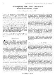
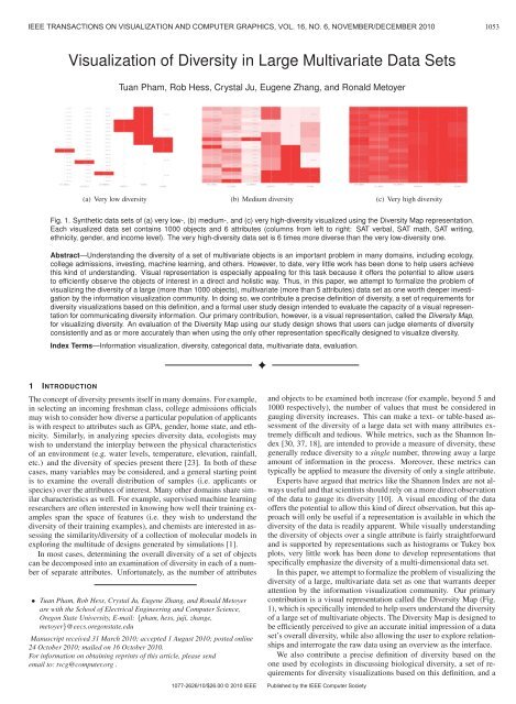
PHAM ET AL: VISUALIZATION OF DIVERSITY IN LARGE MULTIVARIATE DATA SETS1055equally during this process. These techniques are generally applicableto multivariate data sets and offer potential solutions to the diversityvisualization problem. Examples include parallel coordinates [12, 11]and related variants [9, 17], and star coordinates [14].Parallel coordinates [12, 11] are well-suited to visualizing varioustypes of multivariate data (quantitative, ordinal, or nominal) and revealingdata correlation between attributes. However, visual clutterbecomes a limitation as the number of objects increases. Refinementsto parallel coordinates have attempted to address visual clutter withbrushing [9], clustering [3, 7], and dimension reordering [26].Despite these improvements, accurately judging richness of varietyand evenness of abundance may still be difficult using parallel coordinates,especially for larger data sets. However, several variants ofparallel coordinates overcome this limitation by providing informationon the distribution of values for each attribute [9, 17].In one variant, a histogram is overlaid lengthwise on each parallelaxis [9], and bin intervals are created for quantitative attributes bypartitioning them into ranges. Each histogram communicates both therichness of variety and the evenness of abundance of the values of thecorresponding attribute. However, the (necessary) spatial separationof the histograms in this approach may likely affect the user’s abilityto interpret overall diversity without significant effort.The Parallel Sets [17] technique is another variant of parallel coordinatesthat targets categorical data in particular. This representationadopts the layout of parallel coordinates and uses a box to representeach possible value of a categorical attribute. Box size is scaled lengthwisealong the axis in proportion to the frequency of the value in thedata set. Connections between values of two different attributes arealso scaled according to their frequency values. Parallel Sets conveythe distribution of objects over the values of an attribute (i.e. the evennessof abundance for an attribute), as well as relationships betweenthe distributions of values across multiple attributes. However, whilethis approach scales to large data sets, the number of possible attributevalues it can display is limited due to space restrictions. In addition,the boxes corresponding to outliers, i.e. attribute values exhibited byvery few objects, can become imperceptibly small. Moreover, thismethod does not display attribute values not represented in a particulardata set. When combined, these limitations make it very difficultto accurately perceive richness of variety using Parallel Sets.Star coordinates [14] is well-suited to visualizing the overall distributionof a set of objects. Unfortunately, the mapping between adata point and its location in star coordinates is many-to-one. That is,several different data points with equal vector sums will end up in thesame location. This ambiguity makes it difficult to discern richness ofvariety and evenness of abundance over the attribute space.3.3 Icons, Dense Pixels and Stacked DisplaysSeveral other classes of multivariate visualization techniques havebeen developed that are not well suited to diversity visualization. Iconbaseddisplays, such as Chernoff faces [4], typically treat attributes differentlyand as a result, some visual features of the icons (e.g. color)may draw more attention than others, thus violating our requirementof equal consideration for all attributes. Star glyphs, on the other hand,give equal treatment to attributes, however this approach will not scalewell with a large number of objects due to occlusion. While densepixel displays scale well with the number of objects[15], they do notnecessarily display all possible values (only the ones represented inthe data set), making it difficult to gauge richness of variety. Stackeddisplay techniques represent data in a hierarchical fashion and are oftenspace-filling approaches where a hierarchy is nested (or stacked)[20, 31, 13]. Since we are not specifically concerned with hierarchicaldata, these techniques are not considered further.Finally, there is a large group of approaches that fall into the categoryof data preprocessing techniques that generally manipulate thedata to reduce the number of dimensions and/or the number of objects[2, 34, 38]. While these approaches are popular in many domainsas a starting point for exploring data, they typically result in a lossof information and sometimes yield results that are reduced to a nonintuitivespace and are thus difficult for users to interpret, especiallywith respect to the richness of variety. Thus, we do not consider thesetechniques further.3.4 Hybrid TechniquesHybrid techniques integrate multiple visual representations in one ormore windows. The most relevant technique in this class is Pearlmanet al.’s glyph-based approach [25], the only proposed technique to explicitlyaddress the problem of visualizing the diversity of a set of objects.Pearlman et al. focus on communicating both diversity, looselydefined as the distribution of attribute values across a set, as well asdepth, defined as the attribute values of individual members of theset. This technique represents objects as glyphs in a coordinate frame,where three attributes (of possibly many) are used to map objects tothe 2D space of the frame in much the same way as multi-dimensionalobjects are mapped to 2D space using star coordinates (See Figure 3).Other glyph properties, such as shape, size, opacity and color are usedto represent additional attributes and are typically described in an accompanyinglegend. Unfortunately, the number of attributes that canbe successfully encoded using this technique is limited by the perceptualand cognitive loads placed on the user by icon-based approaches.Moreover, the number of objects that can be successfully visualizedusing this technique is limited by occlusion. Nonetheless, this representationis important, since it is the first to explicitly address theproblem of visualizing diversity, and we revisit it in Section 6 wherewe formally compare its ability to communicate diversity informationto that of our Diversity Map representation.4 THE DIVERSITY MAP REPRESENTATIONTo address the shortcomings of previous approaches, we developed anovel representation called the Diversity Map for visualizing the diversityof a set of objects. In this representation, depicted in Fig. 1,each attribute is represented as one of a set of parallel axes, similar tothe parallel coordinate layout. Unlike traditional parallel coordinates,however, each object is represented in the Diversity Map by placing asemi-transparent rectangle on each attribute axis at the locations correspondingto the object’s attribute values. In other words, for a dataset containing N attributes, each object is represented by placing onesemi-transparent rectangle on each of N parallel axes. Note that in ourapproach, we discretize continuous numerical attributes. We refer tothe distinct locations along the attribute axes corresponding to discreteattribute values as buckets.To satisfy the requirement from Section 2 that all objects are treatedequally, each semi-transparent rectangle contributes an equal, fractionalamount of opacity to the bucket in which it is placed. To satisfythe requirement that all attributes are treated equally, we normalize theopacity values on a per-attribute basis so that buckets correspondingto attribute values not represented in the visualized data set are fullytransparent (i.e. α = 0 in RGBA color space), and the bucket(s) correspondingto the most abundant attribute value(s) in the data set arefully opaque (i.e. α = 1). The opacity of every remaining bucket iscalculated based on the ratio of the number of objects in that bucket tothe number of objects in the bucket corresponding to the most abundantattribute value. We have empirically found that using the squarerootof the number of objects per bucket in this calculation helps tomake buckets corresponding to attribute values with low abundancemore recognizable. Specifically, the opacity of each bucket x is calculatedas α(x)= √ |x|/|x MAX |, where |x| denotes the number of objectsin bucket x, and x MAX is the bucket with the most objects for the attributein question. Figure 2 illustrates the process of visualizing asingle attribute using the Diversity Map.An alternative way to view our design is to imagine each attributeaxis as a histogram over the values of that attribute constructed in 3Dspace by stacking semi-transparent tiles on top of each other. Whenviewed from above, the taller stacks of tiles appear darker, while theshorter stacks appear lighter, according to the total combined contributionof the tiles in each stack to that stack’s opacity.

1056 IEEE TRANSACTIONS ON VISUALIZATION AND COMPUTER GRAPHICS, VOL. 16, NO. 6, NOVEMBER/DECEMBER 2010A(0)B(0)C(1)D(0)E(0)A(0)B(0)C(1)D(0)E(1)A(0)B(0)C(5)D(0)E(1)A(0)B(2)C(5)D(0)E(1)A(5)B(2)C(16)D(25)E(7)Start: 1 “C”Add 1 “E” Add 4 “C” Add 2 “B”Add 5 “A”, 11 “C”, 25 “D”, 6 “E”Fig. 2. The process of visualizing a single attribute using the DiversityMap. The depicted attribute has five possible values (A, B, C, D, and E).The visualization begins with a single object with attribute value “C,” andobjects with other attribute values are added in subsequent steps. Ateach step, the number of objects in each bucket is shown in parenthesesnext to the bucket’s label and the opacity (α-value) of each bucket iscalculated as described in the text. Note that, while it is instructive toillustrate the process step-wise, as above, our implementation simplyaggregates object counts and computes opacity values in a single step.Also, note that for a multivariate data set, every object would contributeto each of the parallel attribute axes in the same way as depicted above,resulting in a visualization as depicted in Fig. 1(b).4.1 Design ConsiderationsAs indicated earlier, our primary goal in designing the Diversity Mapwas to make easily apparent the richness of variety and the evennessof abundance of the attribute values exhibited in the data set beingvisualized. While we do not explicitly calculate or assign values forrichness and evenness, we consider them to be quantitative features ofthe data, in that we can think of one data set as being more or less richor even than another. For this reason, we have chosen visual encodingsthat are known to be effective for conveying quantitative information.Specifically, we encode variety using spatial position by assigning adistinct 2D location, or bucket, to each of the possible discrete attributevalues that can be taken by objects in the visualized data set, and weencode abundance using opacity, with each semi-transparent rectanglerepresentation of an object’s attribute value contributing a constant,fractional amount of opacity to the bucket in which it is placed. Underthis encoding, more abundant regions of attribute space are indicatedby visual regions of higher opacity.Because spatial position ranks in the literature as the most effectiveencoding for quantitative information [22, 5], it is easy to justify itsuse in our design. However, several other quantitative encodings, suchas length, angle, slope, and area, rank higher than opacity in [22] and[5]. Unfortunately, these encodings appear to conflict with our chosenspatial encoding. In contrast, we found that opacity serves as anatural complement to the spatial encoding and allows us to elegantlyconvey both the richness of variety and the evenness of abundance ofthe visualized data. In particular, under this combination of encodings,“occlusions” in the 2D visual plane that result from one or moreobjects sharing a certain attribute value serve simply to increase theopacity of that visual region, thereby indicating increased abundance.In the Diversity Map representation, richness of variety is expressedby the number of buckets with non-zero opacity, and evenness of abundanceis expressed by the uniformity of the color distribution acrossthe buckets of a single attribute, as well as over the entire visualization.In other words, the more rich is the variety of a given data set,the more non-transparent buckets it will yield, and the more even isthe abundance across the data set, the more uniform will be the colorsof the buckets.The overall diversity of a given data set—that is, the combined diversityof all its attributes—is communicated by the Diversity Map asthe overall color density of the entire visual region: as the visualizeddata set becomes more richly various and more evenly abundant, morebuckets will exhibit a similar non-transparent color. In the limit of“perfect” diversity, where all possible values of each attribute are representedequally, the entire visual region will be a solid, completelyopaque color. Conversely, a set with little diversity will produce a visualizationwith regions of very high contrast. As examples of thesephenomena, consider the synthetic data sets with zero and near-perfectdiversity visualized using a Diversity Map in Figs. 1 (a) and (c).Finally, we note that the Diversity Map is specifically designed toprovide a holistic overview of the population sample of interest. AsShneiderman notes, [32], providing an overview of the data is an importantpart of a visualization system, as overviews help the user builda mental model of how the data covers the attribute space. This modelin turn helps the user formulate actions such as queries [28]. Indeed,a good overview representation should serve as a gateway by allowingthe user to interact with the visualization in order to investigatethe data based on the mental model he or she has formed. While wereserve deeper investigation of this matter for future work, we simplynote that the Diversity Map is designed to serve as just such a gateway.5 USER STUDY DESIGNIn this section, we describe a formal user study designed to measure agiven visualization’s ability to communicate diversity information. Inparticular, the study is a controlled user study intended to be conductedin a laboratory setting, and it is designed to compare the visualizationof interest against a given baseline visualization. There are two importantcomponents to this design: 1) a method for generating syntheticdata sets with controllable, varying levels of diversity and 2) a set ofquestions, each of which is meant to assess a study participant’s abilityto comprehend a particular aspect of diversity using each of thevisualizations under comparison. We describe these components next.5.1 Synthetic Data GenerationWhile, ideally, we would use a real data set to evaluate a visualization,we require data with specific distributions of values over attributes.Since it is difficult to find data sets that can accommodate this requirement,we developed a technique for creating synthetic data setsof controllable, varying diversity over a set of independent attributes.In particular, our procedure generates synthetic sets of objects overa manually defined set of attributes and attribute values, where therichness of variety and evenness of abundance over each attribute iscontrolled and measured.Our data generation procedure is based on the Shannon index, orShannon entropy, a measure of diversity that is widely used in ecology[30, 37, 18]. Shannon entropy is also used in other fields, such asinformation theory, where it is used to measure the amount of informationcontained in a coded message. In its general form, the entropy ofa single random variable, X (in biodiversity, X corresponds to species;in the more general case, it could correspond to any single attribute) isSH(X) =− ∑ p(x i )log p(x i ), (1)i=1where {x 1 ,...,x S } is the set of possible values of X and p(x i ) isthe probability that X takes value x i . In biodiversity, for example,x 1 ,...,x S represent the possible species and p(x i ) represents the probabilityof observing one particular species x i . In practice, we computep(x i ) as the ratio of the number n i of instances of value x i to the totalnumber N of individuals in the set, i.e. p(x i )= n iN . In other words,p(x i ) represents the relative abundance of value x i in the total set.H(X) is directly proportional to the level of diversity within a singleattribute, in that higher values of H(X) correspond to richer variety andmore even abundances. Unfortunately, it is difficult to compare valuesof H(X) across attributes, since it is scaled to the number of possiblevalues of the attribute being measured. This implies that an attributewith many possible attribute values (e.g. the home state of a student)may be considered more diverse under entropy than an attribute withfew possible values (e.g. the gender of a student), even if it is not.In order to meet our requirement from Section 2 that all attributesare considered as equal, we have adapted a variant of the Shannonindex known as the evenness measure [27], which normalizes the valueof H(X) by its maximum possible value:S 1H max (X) =− ∑i=1 S log 1 = logS. (2)S

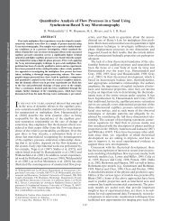
PHAM ET AL: VISUALIZATION OF DIVERSITY IN LARGE MULTIVARIATE DATA SETS1057Thus, the evenness of attribute X isH E (X) =H(X)H max (X) = − 1logSS∑ p(x i )log p(x i ). (3)i=1Note that, despite its name, this measure captures both the richnessand evenness of attribute X. In particular, richness, which measuresthe number of values of represented out of all possible values of X, isindicated by the number of values x i with non-zero probability. Themore of these that are present for attribute X, the higher the valueof H E (X). Likewise, evenness is indicated by the uniformity of theprobabilities p(x i ), and H E (X) is maximized when each attribute valuex i occurs with the same probability. An important property of thismeasure is that it always takes a value between 0 (zero diversity) and1 (full diversity).In our setting, we have one variable X k corresponding to each attribute,and we hand-specify the possible values {xi k}Ski=1 for each attributeX k . We model the distribution p(xi k ) over the possible valuesof each attribute as multinomial. In other words, associated with eachpossible attribute value xi k is a weight wk i , where wk i ≥ 0 for i = 1,...,S kand ∑ i w k i = 1, and the attribute values in a given set are distributed inproportion to those weights.To rigorously test visualization methods, we wish to be able to generatedata that achieves a pre-specified target value HE ∗(Xk ) of theevenness measure for each attribute X k . We model this as a set ofseparate non-linear optimization problems, one for each attribute. Theobjective for each problem is to find the set of weights {w k i }Sk i=1 thatminimizes the squared error between the resulting evenness H E (X k )and the target evenness HE ∗(Xk ). We solve for these weights using agradient-based quasi-Newton method.Once the distribution p(xi k) is instantiated with weights {wk i }Sk i=1for each attribute X k , we generate synthetic data by simply drawingsamples from each of these distributions and using the j th sample foreach attribute as the corresponding attribute value of the j th object inthe data set. Then we use H = ∑ k H E (X k ) as a measure of the overalldiversity of a particular data set.5.2 User Study QuestionsOur user study contains four types of questions. Each type is designedto assess a different aspect of the user’s ability to perceive diversityusing a particular visualization. We outline each question type here.Q1: Between two visualizations generated with the same method,which picture represents a more diverse set of objects? (possible answers:picture A or picture B) The primary goal of this question typeis to determine if a visualization technique is discriminative enough toallow a user to distinguish and compare the levels of overall diversitydepicted in two visualizations generated with the same technique. Thedifficulty of each question of this type can be determined by the differencein the overall diversity values H between two visualized datasets. The bigger this difference, the easier the question is.Q2: How diverse is the data set represented in this picture? (possibleanswers: very low diversity, low diversity, medium diversity, highdiversity, very high diversity) This question type is intended to identifyhow well a user can interpret and assign a diversity value to a visualizationgiven baseline examples of zero and full diversity (which weprovide to users in tutorials; see Section 6). The level of diversity of adata set is determined based on its overall diversity value H.Q3: What is the most/least diverse attribute in the data set representedin this picture? (possible answers: the possible attributes)This question type is designed to understand the participant’s abilityto identify relative differences in diversity among attributes that mayhave different levels of richness of variety or evenness of abundance.The difficulty of each question of this type can be determined by thedifference between the values of the evenness measurements H E (X k )of the most/least and second-most/least diverse attributes. The biggerthis difference, the easier the question is.(a) (b) (c)Fig. 3. Synthetic data sets of (a) very low-, (b) medium-, and (c) veryhigh-diversity visualized using the Glyph Hybrid (GH) representation(the accompanying legend is not shown). Each visualized data set contains1000 objects and 6 attributes (SAT verbal, SAT math, SAT writing,ethnicity, gender, income level). The SAT attributes are mapped tothe 3 coordinate axes. Ethnicity, gender, and income are mapped tocolor, shape, and size of the glyphs respectively. Additionally, opacityencodes composite SAT scores (as in Pearlman’s implementation) toremedy ambiguity caused by the many-to-one mapping. The very highdiversity data set is 6 times more diverse than the very low data set.The data sets are identical to the ones in Fig. 1.Q4: Which value of attribute X contains the most/least objects?(possible answers: possible values of attribute X) The last questiontype is designed to determine the participant’s ability to isolate attributevalues with high and low relative abundance of objects, givena particular attribute to inspect (e.g. ethnicity). The difficulty of eachquestion of this type can be determined by the difference between thenumber of objects exhibiting the most/least abundant attribute valueand the number exhibiting the second-most/least abundant attributevalue. The bigger this difference, the easier the question is.In a study, questions of each question type are the same in terms ofwording. However, they can be asked multiple times on different datasets to vary the difficulty (Q1, Q3, Q4) or the level of diversity (Q2).For each of these question types, ground-truth answers are based onthe distribution of objects and the evenness measure values obtainedusing our synthetic data generation method.6 EVALUATION OF THE DIVERSITY MAP REPRESENTATIONIn this section, we use the formal user study described in the previoussection to evaluate the effectiveness of the Diversity Map representation(DM; Fig. 1) at conveying diversity information by comparing itto the Glyph Hybrid representation [25] (GH; Fig. 3) discussed in Section3. We chose GH as the baseline for this comparison because it isthe only previous method developed specifically to visualize diversity.Nevertheless, in the future work, it will be informative to compare DMwith other traditional small multiples, such as multiple histograms.Here we describe the specific implementation of the user study outlinedin Section 5 that we used to compare the DM and GH representations,and we analyze and discuss the results of this study.6.1 User Study ImplementationData. The synthetic data sets we used in our user study simulatedcollege applicant pools where the objects are applicants characterizedby the following six attributes:• SAT Verbal Score: 200-800, discretized by steps of 30• SAT Math Score: 200-800, discretized by steps of 30• SAT Writing Score: 200-800, discretized by steps of 30• Ethnicity: B, H, I, O, W, or X• Gender: F or M• Income: Bracket 0, Bracket 1, Bracket 2, Bracket 3, or Bracket 4We chose the college applicant domain because it is one of the threedomains examined as a case study by Pearlman et al. in [25] and becausewe believed it would be a domain with which our participants,who were all university students, would be familiar.Participants and Protocol. The participants in our study were 40students at our university, all with normal color vision. All of the participantsvolunteered to participate in our study in response to fliers

1058 IEEE TRANSACTIONS ON VISUALIZATION AND COMPUTER GRAPHICS, VOL. 16, NO. 6, NOVEMBER/DECEMBER 2010Fig. 4. Participants of the user study visualized using Diversity Map.The visualized attributes, from left to right, are major, degree, year inschool, gender, and age-range. The participants represented a diverserange of majors, degrees, and ages.Table 1. Allocation of 40 participants across 4 treatments. E.g., 10 (DM,A)–(GH, B) indicates 10 participants answered questions on collectionA with DM in phase 1 then on collection B with GH in phase 2.10 (DM, A)–(GH, B) 10 (DM, B)–(GH, A)10 (GH, B)–(DM, A) 10 (GH, A)–(DM, B)posted around the campus. They represented a diverse range of majors,degrees, and ages (Fig. 4), and, although their participation in ourstudy might indicate interest in diversity visualization, most of the participantswere unfamiliar with the field of information visualization.After the signing of an informed consent document required byour university’s Institutional Review Board, each participant was randomlyassigned to different experimental conditions as described below.Participants were encouraged to ask any questions they mighthave at any time during the course of the study.Experiment Design. We followed a two-phase crossover experimentdesign and used two collections of synthetic data sets, collectionA and collection B, for the two phases to avoid learning effect whenparticipants moved from one visualization method to the other. Notethat both data set collections are considered equivalent in all respects.They were simply generated with separate runs of the data generationalgorithm described in Section 5.1.Each participant’s session was divided into two phases. In the firstphase, the participant answered questions about visualizations of onecollection of data sets created with one visualization method. In thesecond phase, the participant answered the same questions about visualizationsof the other collection of data sets using the other visualizationmethod. The order of visualization methods and data set collectionswas counter-balanced across participants (see Table 1).In each phase, the participant first completed a short tutorial thatexplained the visualization method involved in the phase and includedseveral example images generated using that method. After completingthe tutorial, the participant answered several questions of each ofthe types described in Section 5. Note that participants were suppliedwith a hard copy of each tutorial to consult while answering thesequestions. Note also that the questions of one type are the same, buteach one is asked about visualizations of different data sets. The orderingof question types was randomized across two phases and acrossparticipants, but all questions of the same type were asked as a block.Each participant answered six questions of type Q1. A secondarygoal for this question type was to determine whether data set size affectedparticipants’ ability to judge and compare overall diversity levels.Thus, each participant was asked Q1 questions of three levels ofdifficulty (easy, medium, hard) for each of two different data set sizes(100 and 1000 objects). Half of the participants answered questionsusing the smaller data sets first and the larger ones second, and theother half answered questions using the larger data sets first and thesmaller ones second. The order of the three difficulty levels was randomizedwithin each data set size for each participant. This orderingconvention was chosen to avoid ordering effects among participants.Each participant answered three questions of type Q2, and six questionseach of types Q3 and Q4. To avoid ordering effects for thesequestions, we used a counterbalancing/randomization approach similarto the one used with Q1 questions. For all of these questions, weused data sets with only 100 objects. Though our goal is to developvisualizations that can handle data sets with more that 1000 objects,we believed that GH would suffer with larger data sets because of occlusion/clutter.To compare the capabilities of the respective methodsto effectively communicate information about diversity, we used datasets with only 100 objects so as not to disadvantage GH.We collected answers to these questions not only to measure absolutecorrectness but also to identify how far each participant’s responsewas from the correct answer. We accomplished this by assigning anerror distance to each response. For questions of type Q1, correct responseswere assigned an error distance of 0, while incorrect responseswere assigned an error distance of 1. For questions of type Q2, Q3,and Q4, the error distance of each response was computed as the rankorder of the participant’s selected response in relation to the correctanswer. In particular, the best (correct) answer was assigned an errordistance of 0, the second-best answer was assigned an error distance of1, the third-best answer was assigned an error distance of 2, and so on.As an example, consider a question of type Q2 whose correct answerwas “low diversity.” For this question, a response of “very low diversity”would be assigned an error distance of 1, as would a responseof “medium diversity,” while a response of “high diversity” would beassigned an error distance of 2, and a response of “very high diversity”would be assigned an error distance of 3. We used a similar system toassign error distances for questions of type Q3 and Q4 based on thediversity ordering of the attributes and the cardinality ordering of theattribute values, respectively.We also collected response times in addition to error distances. Participantswere given a time limit of two minutes to answer each question.If the participant did not answer the question in the allotted time,the system timed out and sent the participant to the next question. Theparticipant was assigned the maximum possible error distance for thequestion type for any question on which he or she timed out.In addition to the questions of type Q1-Q4, at the end of each phase,the participants answered a short questionnaire about their experiencewith each method. This questionnaire contained both Likert-stylequestions as well as open-ended questions. We discuss these questionsin more detail in our analysis of the study results below.The entire study was administered through a web-based interfacethat collected demographic information, presented tutorials and questions,collected user answers, computed error distances and responsetimes, and stored these in a database for analysis. The resolution ofthe monitor used for all studies was the standard 1920 × 1200 pixels.The resolution of each image produced by the DM visualization was900×537 pixels, and the resolution of each image produced by the GHvisualization was 640 × 640 pixels. Each question for the GH methodrequired a legend image of 200×524 pixels. When the legend is takeninto account, visualizations of both methods are roughly the same size.6.2 Results and AnalysisHere, we analyze the results obtained from the user study. Our initialhypothesis about these results was that, for each question type, DMwould outperform GH, both in terms of accuracy and response time.In particular, we believed that GH would suffer for some questionsdue to the fact that it does not treat all attributes as equal. Specifically,we expected users to have difficulty accurately judging diversity forthe attributes mapped to GH’s three spatial axes, due to the ambiguousmany-to-one mapping these axes produce. We also expected GH tosuffer in terms of time and/or accuracy due to the need for users toconsult the legend to remember the mappings.For each question type, we did not analyze individual answers butcomputed the sum of error distances and the sum of response timesacross the questions of that type for each participant and comparedthe distributions of these aggregated values using statistical hypothesistesting. While we initially planned to use ANOVA and repeatedmeasuresANOVA directly for this comparison, we found that the responsedata did not meet these methods’ normality requirements. Wetherefore first applied a rank transformation [6] to the response databefore using these techniques.Our primary focus in analyzing the results of the study is on error

PHAM ET AL: VISUALIZATION OF DIVERSITY IN LARGE MULTIVARIATE DATA SETS1059Table 2. Mean sum of error distances for each question type as a function of visualization method (DM or GH), collection of data sets (A or B), andphase (P1 or P2). Standard deviations are shown in parentheses. The table structure is split by collections of data sets because our preliminaryanalysis showed that the collection of data sets had a statistically significant effect on the error distance for method GH.QuestionQ1Q2Q3Q4MethodCollection ACollection BP1 P2 P1&2 P1 P2 P1&2GH 0.50 (0.71) 0.40 (0.52) 0.45 (0.60) 0.90 (0.74) 1.40 (0.70) 1.15 (0.75)DM 0.60 (1.07) 0.30 (0.48) 0.45 (0.83) 0.50 (0.53) 0.60 (0.70) 0.55 (0.60)GH 2.70 (1.25) 3.70 (1.06) 3.20 (1.24) 2.00 (0.94) 2.40 (0.97) 2.20 (0.95)DM 2.10 (1.66) 1.70 (0.67) 1.90 (1.25) 1.70 (0.67) 2.10 (0.74) 1.90 (0.72)GH 16.10 (2.02) 15.70 (3.09) 15.90 (2.55) 9.10 (3.31) 9.30 (2.98) 9.20 (3.07)DM 3.60 (4.53) 3.50 (4.88) 3.55 (4.58) 5.50 (3.27) 4.70 (4.03) 5.10 (3.60)GH 2.20 (1.40) 1.20 (1.40) 1.70 (1.45) 2.90 (1.60) 3.10 (2.02) 3.00 (1.78)DM 0.50 (1.27) 1.90 (3.38) 1.20 (2.59) 0.70 (1.89) 3.30 (8.27) 2.00 (5.99)Table 3. Mean sum of response times (in seconds) for each question type as a function of visualization method (DM or GH), phase (Phase 1 orPhase 2), and collection of data sets (A or B). Standard deviations are shown in parentheses. The table structure is split by phases because ourpreliminary analysis showed statistically significant evidence of an effect of phase of method on response time for DM.QuestionQ1Q2Q3Q4MethodPhase 1 Phase 2A B A&B A B A&BGH 114.40 (53.74) 120.50 (66.44) 117.50 (58.90) 105.70 (53.22) 93.40 (37.66) 99.55 (45.31)DM 151.60 (88.32) 121.90 (44.42) 136.80 (69.73) 79.40 (37.89) 91.20 (24.05) 85.30 (31.48)GH 53.90 (37.73) 56.00 (21.29) 54.95 (29.84) 41.20 (23.19) 50.00 (23.75) 45.60 (23.29)DM 66.90 (26.54) 53.60 (15.21) 60.25 (22.13) 38.70 (31.73) 43.20 (17.85) 40.95 (25.16)GH 179.70 (61.18) 208.40 (85.49) 194.10 (73.84) 216.50 (61.67) 180.80 (46.88) 198.70 (56.37)DM 143.60 (43.96) 153.30 (43.21) 148.40 (42.72) 98.50 (34.95) 105.30 (29.61) 101.90 (31.72)GH 130.50 (44.94) 118.00 (34.91) 124.20 (39.69) 97.10 (18.88) 108.10 (55.89) 102.60 (40.99)DM 93.40 (42.86) 120.90 (76.02) 107.20 (61.70) 86.10 (43.18) 53.40 (23.33) 69.75 (37.71)distance, since we believe this is the most important performance measurefor a given representation. However, we still pay close attention toresponse time, as well. In all cases, our null hypothesis is that no differenceexists between the distributions of corresponding performancemeasures across the methods DM and GH.We chose a two-phase crossover experiment design in order to reducethe number of participants and to keep individual subject variabilitylow. However, the design also required us to account for additionalwithin-subjects factors, namely, phase of method (first or second) andcollection of data sets (A or B). While we did not expect either ofthese factors to have a statistically significant effect on our results, thiswas not the case. Our preliminary analysis showed that the collectionof data sets had a statistically significant effect on the error distancefor method GH. This effect was not statistically significant for DM.As a result of this effect we analyze error distance separately for eachcollection. In addition, our preliminary analysis showed statisticallysignificant evidence of an effect of phase of method on response timefor DM. Specifically, participants performed slightly faster with DMin the second phase of the study than in the first phase. Interestingly,there was no significant evidence for this effect for GH. Regardless,due to this effect, we analyze response time using only data collectedduring the first phase of participants’ sessions. Tables 2 and 3 respectivelysummarize the error distance and response time results.Analysis of Results for Q1. Between two visualizations generatedwith the same method, which picture represents a more diverse setof objects? As Table 2 indicates, participants answered Q1 questionsmore accurately with DM than with GH, particularly for collection B.In fact, there is convincing statistical evidence for an effect of visualizationmethod on error distance with collection B, F(1,38) =7.53,p = 0.009. However, with collection A, there is no evidence of suchan effect, F(1,38) =0.21, p = 0.65. These results hold consistentwhen analyzing data separately over 100 and 1000 object data sets,suggesting no effect of data set size on accuracy for questions of thistype. With regard to response time, though Table 2 suggests that participantsperformed slightly faster using GH in phase 1, the evidencefor this effect is not statistically significant, F(1,38)=1.20, p = 0.28.While these results do not support our initial hypothesis that userswould perform more quickly when using DM than when using GH,they do substantiate our hypothesis that users would be able to moreaccurately compare the diversity of two data sets when using DM thanwhen using GH. Examining these results more closely, we found thatmuch of the difference in performance between collections A and Bfor participants using GH was accounted for by the fact that many participants(13 out of 20) incorrectly answered one particular questionof medium difficulty from collection B using GH. In this question, thedata set with lower overall diversity contained a very diverse Ethnicityattribute, while the data set with higher overall diversity containeda very diverse Gender attribute but a much less diverse Ethnicity attribute.In GH, the Ethnicity attribute is mapped to glyph color andthe Gender attribute is mapped to glyph shape. We believe that inanswering this question, participants placed more weight on the distributionof color in the visualization than on the distribution of shape,misleading them into an incorrect judgment of overall diversity. If thisexplanation is correct, it points to an interesting consequence of GH’sunequal treatment of attributes. DM, on the other hand, does not seemto suffer from this consequence because it treats all attributes as equal.Analysis of Results for Q2. How diverse is the data set representedin this picture? The results for Q2 were similar to Q1’s, withparticipants tending to judge absolute levels of overall diversity moreaccurately with DM. Again, with GH, users’ performance dependedheavily on data set collection: participants using GH performed worseon collection A than on collection B. In fact, for collection A, therewas convincing evidence for an effect of visualization method on errordistance, F(1,38) =15.02, p = 0.0004. For collection B, there wasnot statistically significant evidence for this effect, F(1,38) =1.56,p = 0.22. Again for Q2, there was no evidence for an effect of methodon response time in phase 1, F(1,38)=1.91, p = 0.18.These results, too, do not support our initial hypothesis that userswould perform more quickly when using DM than when using GH,but they do sustain our hypothesis that users would be able to moreaccurately assign an absolute diversity value to a given data set whenusing DM than when using GH. Again, more closely examining theseresults, we found that the three data sets used for Q2 questions fromcollection A (low, medium, and very high diversity) tended to be morediverse than the corresponding data sets from collection B (very low,medium, and high diversity). With this in mind, we suspect that participantsmay have been more hesitant to choose a higher diversity responsewhen using GH than when using DM, perhaps because, while itis clear what very low overall diversity looks like under GH (very fewspatial locations, colors, shapes, etc.; see Fig. 3(a)), what very high

1060 IEEE TRANSACTIONS ON VISUALIZATION AND COMPUTER GRAPHICS, VOL. 16, NO. 6, NOVEMBER/DECEMBER 2010overall diversity looks like under GH is much more ambiguous (evenly“spread out” glyphs with evenly distributed colors, shapes, etc.; seeFig. 3(c)). On the other hand, using DM, it was likely much easier forparticipants to understand exactly how very low and very high diversityappear visually (very low and very high total color density of theentire visual region, respectively; see Figs. 1 (a) and (c)), and we believethis led them to be more confident in choosing responses at bothends of the diversity spectrum when using DM for Q2 questions.Analysis of Results for Q3. What is the most/least diverse attributein the data set represented in this picture? The results for Q3 verymuch favored DM. There was convincing evidence for an effect of visualizationmethod on error distance for both collections of data sets,A and B, F(1,38)=75.54, p = 1.45 × 10 −10 and F(1,38)=13.565,p = 0.0007, respectively. In addition, there was suggestive but inconclusiveevidence for an effect of visualization method on response timein phase 1, F(1,38)=3.50, p = 0.07. These results appear to confirmour initial hypothesis that users would perform better—both in termsof error distance and response time—when making judgments aboutthe diversity of a single attribute when using DM than when using GH.Interestingly, participants using GH appeared to perform worse onQ3 questions where the correct answer was an attribute assigned to aspatial axis, likely due to GH’s ambiguous many-to-one spatial mapping.In contrast, participants using DM did not appear to favor anysingle attribute for questions of this type. Again, this suggests thatDM’s treatment of all attributes as equal is one of its strengths.Analysis of Results for Q4. Which value of attribute X contains themost/least objects? As with Q3, the results for Q4 very much favoredDM. For questions of this type, there was convincing evidence for aneffect of visualization method on error distance for both collections ofdata sets A and B, F(1,38)=7.58, p = 0.009 and F(1,38)=25.18,p = 1.26 × 10 −5 , respectively, and there was suggestive but inconclusiveevidence for an effect of visualization method on response time inphase 1, F(1,38) =2.61, p = 0.11. Again, these results support ourinitial hypothesis that users would be able to more quickly and moreaccurately make judgments about relative abundances within a singleattribute when using DM than when using GH.Summary. The results across Q1–Q4 consistently supported ourhypothesis that users would be able to make more accurate judgmentsabout various aspects of the diversity of data when using DM thanwhen using GH. While we found some evidence suggesting that usersperformed more quickly with DM than with GH, these results werenot conclusive. Similarly, we found no conclusive evidence that sizeof data set had an effect on user performance for questions of type Q1.6.3 Subjective EvaluationAfter each participant answered all of the questions of types Q1–Q4for a particular method, he or she also completed a short questionnaireon that method. The questionnaire, whose form we adopted from[33], consisted of nine Likert-style statements, where participants wereasked to indicate their level of agreement on a scale of 1 (strongly disagree)to 5 (strongly agree), and three open-ended questions.Table 4 lists each of the Likert-style questions along with the participants’mean responses for both GH and DM. Participants slightlyfavored DM over GH in making judgments of diversity componentsand this is consistent with their performance in the objective portionof the study. Participants also slightly favored DM over GH in termsof applicability, ease of understanding, and affinity.In addition to the Likert-style statements, the questionnaires includedthe following three open-ended questions:O1) What aspect(s) of this method did you like most?O2) What aspect(s) of this method did you dislike most?O3) If possible, how would you change this method to improve it?Many participants indicated an affinity for GH because it was intuitive,in that, as the diversity of the underlying data increased, sotoo did the diversity of the visual properties (color, shape, size, etc.)of the generated visualization. On the other hand, many participantsexpressed concern about GH’s ambiguous spatial layout, which theyfound confusing.Table 4. Mean responses to each of nine Likert-style statementspresented to participants immediately after using each visualizationmethod. These responses are based on a scale of 1 (strongly disagree)to 5 (strongly agree). Standard deviations are shown in parentheses.Statement GH DML1) I was able to compare the diversity of two data 3.75 (0.81) 3.93 (0.92)sets using this method.L2) I was able to judge the diversity of a single 3.63 (0.90) 4.25 (0.84)data set using this method.L3) I was able to determine the most/least diverse 3.58 (0.96) 4.15 (0.86)attributes in a data set using this method.L4) I was able to determine the ethnicity with the 4.05 (0.88) 4.28 (0.82)most/least objects using this method.L5) After the initial training session, I knew how 3.33 (0.83) 3.55 (0.99)to use this method well.L6) After answering all of the questions, I knew 3.74 (0.88) 3.88 (0.91)how to use this method well.L7) There are definitely times that I would like to 3.20 (1.04) 3.75 (0.93)use this method.L8) I found this method to be confusing. 3.38 (1.21) 2.77 (1.13)L9) I liked using this method. 2.95 (0.96) 3.50 (1.01)Participants indicated that they liked the “clean layout” of DM; thesimplicity of comparing color opacity under DM; and its ability toeasily handle different data set sizes. On the other hand, some participantsdisliked comparing the diversity of an attribute with severalbuckets (e.g. ethnicity) to that of an attribute with only a few buckets(e.g. gender). Interestingly, though this appears to be an issue with GHas well, participants did not seem to notice it when using GH.Finally, most participants (29 out of 40) preferred DM to GH. Ingeneral, participants tended to feel GH would be best suited for judgingthe overall diversity of a data set, especially to determine if the setis not diverse. Interestingly, this is in direct contradiction to their performancein questions Q1 and Q2 which favored DM. In contrast, participantsgenerally believed DM would be useful for investigating thedata more deeply and examining the diversity of individual attributes.7 DISCUSSION AND FUTURE WORKWe have presented 1) an infrastructure for studying the problem of diversityvisualization and 2) a novel representation for visualizing thediversity of a large set of multivariate objects. The infrastructure includesa precise definition of diversity that takes both richness andevenness into account, a method for generating synthetic data of controllablelevels of diversity, and a formal study design for evaluatingdiversity visualization representations. Based on this definition andstudy design, we developed and evaluated our approach to diversityvisualization, the Diversity Map, which is based loosely on ideas fromboth parallel coordinates and small multiple histograms. We show thatthe Diversity Map allows users to consistently and as or more accuratelyjudge elements of diversity than the only other existing methoddesigned to visualize diversity. While we believe we have taken apositive step in understanding diversity visualization, there are severalissues left to address.Study Design Issues. First, while our study design focuses on staticvisualizations only, both DM and GH are interactive visualizations.We avoided interactive features to limit the scope of our study to firstunderstand the merits and shortcomings of DM and GH as representations.Future work will address the interactive capabilities of DM.Additionally, implementing GH required us to choose a mappingof attributes to the various visual properties of the representation (thethree spatial axes, color, size, shape, etc.). While we based our mappingon the one used by Pearlman et al. [25], our choices here nonethelessrepresent a possible threat to construct validity.Finally, our study does not include a specific question to determinethe richness of variety of an attribute. At first glance, it would appearthat richness of variety was obvious in both methods. However,while richness is clearly communicated in DM and in the non-spatialattributes of GH (e.g. color, shape, size), it is not clear how well richnessis communicated in the spatial axes of GH (e.g. the richness of

PHAM ET AL: VISUALIZATION OF DIVERSITY IN LARGE MULTIVARIATE DATA SETS1061SAT scores in Figure 3 is ambiguous). The evaluation study wouldbenefit from explicit attention to the ability to communicate richness.Limitations of DM. The Diversity Map representation (DM) itselfis also not without limitations. First, DM is currently designed to visualizeonly categorical data, requiring a discretization of quantitativeattributes. Second, the static visualization provides limited insight intothe relationships between attributes. However, variations on the interactiveversion of DM can address these problems. For example, traditionalparallel coordinates poly-lines can be selectively displayed overDM to allow the user to view the actual quantitative attribute values.These poly-lines also allow the user to see and select individual objects,which are currently not visible in the static DM visualization aspresented. Filtering techniques are also implemented in the interactiveversion of DM to allow users to perform queries. For example, theuser can constrain a single attribute to one or more particular values(buckets) using the mouse. The remaining attributes then display thediversity of only those objects that fall within the specified range of thefiltered attribute. With filtering, users can answer questions regardingthe relationship between two attributes such as “In what bucket in attributeX are objects most/least diverse in attribute Y?”.In future work, we will explore other interaction features includinguser-defined orderings for nominal-valued attributes, user-definedordering of the attribute axes themselves, and user specification of attributevalue ranges (over multiple buckets) of interest for interactivefiltering. In addition, we plan to investigate mechanisms for constructingsets of objects of a desired diversity. Finally, we also plan to explorethe advantages of small multiples of DMs for trend analysis.While the Diversity Map representation scales well with the numberof objects to be visualized, like many multivariate visualization methods,scaling with an increase in attributes is limited by screen space.Likewise, the number of buckets for any one attribute is also similarlylimited, and it is not clear how “small” a bucket can be made beforethe representation becomes ineffective. Studies to understand theselimitations are left for future work.The Diversity Map representation, like many others, requires initialtraining for users to be effective in reading the visualization. Indeed,many pilot users of the visualization found the representation counterintuitive.They assumed that if a representation is to convey diversity,high diversity should be shown with an image in which all of the objectslook different, however, in our implementation, high diversity resultsin a uniform image (see Fig. 1(c)). This confusion stems from theusers associating each box with an individual object to be visualized.Once users understood that DM did not display individual objects, butrather their distribution over the attribute space, they were much morereceptive and able to interpret the visualizations consistently as shownin the study. We believe that this representation, where the space fillingeffect denotes diversity, helps the user establish a baseline for highdiversity. In fact, this is supported by the results of our formal study.While participants tended to underestimate diversity when using theGH method, where more diversity implies more dissimilar symbols,they were able to more accurately assign absolute diversity values aswell as compare diversity between two data sets using DM.Note that we empirically chose white as the background color andred as the foreground color in DM. However, we have since foundstudies indicating that blue may be a more appropriate foregroundcolor, since our eyes are known to be more sensitive to changes inblue than in red [21]. Additionally, we empirically used the squareroot-based normalization in determining the color opacity (α-value)of buckets to help make buckets corresponding to attribute values withlow abundance more recognizable. Nevertheless, this ad-hoc scalingfactor is not necessarily a preferred choice by all users. In fact, ecologistsmay prefer a log transformation to accommodate species whoseabundances span multiple orders of magnitude [23]. Moreover, wecould employ an alternative to the RGBA color space, such as CIElabor CIEluv, which are perceptually uniform color spaces and may bemore appropriate for representing quantitative abundances [36].Limitations of our definition of diversity. Our definition of diversitygeneralizes the one used in the field of Ecology to the case ofarbitrary multivariate data. As a consequence our definition looks atFig. 5. A real data set of 2550 college applicants with 10 attributesvisualized using the Diversity Map. Left: the subset of students recommendedfor acceptance based on a holistic admissions process implementedby a proprietary software package and designed to producea diverse incoming class. Right: the subset of rejected students. Therecommended students yield a visualization with a more even distributionof opacity, especially in attributes like GPA, ethnicity, residency, andmajor (columns 1, 4, 6, and 8 respectively). This suggests that the recommendedapplicants are more diverse than the rejected ones.the diversity of each attribute independently and does not take into accountthe interaction between attributes. In future work, we will investigatea definition to account for this interaction. The area of businessmanagement may provide useful insights as researchers in that fielddiscuss diversity across multiple attributes [19, 8].Application to Real Data. We also intend to explore the applicationof Diversity Maps to real-world data. As an example, we appliedDiversity Maps to a real data set containing 2550 applicants (one yearworth) to a particular university. Each applicant is characterized byten attributes. Interestingly, this real data set was preprocessed usingan existing proprietary software package designed to recommend a setof applicants using a holistic evaluation process intended to producea diverse incoming class. The DM visualizations of this data set areshown in Fig. 5. These results are promising in that they agree withthe output of the holistic evaluation software.We are also in the process of deploying an interactive version ofthe Diversity Map for use by ecologists at our university. Ecologistscommonly collect species inventory data and analyze it to better understandthe interactions between the environment and the species understudy. For example, species distribution modeling is used to relateenvironmental covariates to each species. Data sets of this type areoften challenging in many ways. In the Oregon State University H.J.Andrews Experimental Forest, researchers have collected data on 606moth species by sampling ∼200 sites across a ∼100 km 2 region ofstudy every summer week over a period of 23 years [24]. This data isinteresting because moths are indicators of broader biological diversityin plant types and physical environments. Diversity measures such asthe Shannon Index provide little insight into relationships that may bepresent in this data between the species and the environment because,in reducing diversity to a single number, they conceal a tremendousamount of information.8 CONCLUSIONSThe Diversity Map represents a first attempt to design a representationwith the specific goal of visualizing diversity as we have definedit in this paper. While, to date, little attention has been paid to thisproblem, we hope that this work will serve to provide a foundation forfuture studies into the design and evaluation of visualization methodsfor exploring the increasingly important area of diversity.ACKNOWLEDGMENTSThe authors wish to thank Onyekwere Ogba and Nicholas Hubbert fortheir development efforts supported in part by the CRA-W/CDC DistributedResearch Experiences for Undergraduates (DREU) program.In addition we would like to thank Dr. Margaret Burnett, Dr. JuanGilbert, Dr. Julia Jones, Dr. Jeff Miller, and Steven Highland for numerousdiscussions regarding our user study, application to admissionsdata, and application to moth diversity data. Finally we would like tothank our user study participants for their time and input. This workwas supported in part by NSF IIS-0546881.

1062 IEEE TRANSACTIONS ON VISUALIZATION AND COMPUTER GRAPHICS, VOL. 16, NO. 6, NOVEMBER/DECEMBER 2010REFERENCES[1] A method for quantifying and visualizing the diversity of qsar models.Journal of Molecular Graphics and Modelling, 22(4):275 – 284, 2004.[2] T. Anderson. An introduction to multivariate statistical analysis. WileyNew York, 1958.[3] A. Artero, M. de Oliveira, and H. Levkowitz. Uncovering clusters incrowded parallel coordinates visualizations. In Proceedings of the IEEESymposium on Information Visualization, pages 81–88. IEEE ComputerSociety, 2004.[4] H. Chernoff. The use of faces to represent points in k-dimensional spacegraphically. Journal of the American Statistical Association, pages 361–368, 1973.[5] W. Cleveland and R. McGill. Graphical perception: Theory, experimentation,and application to the development of graphical methods. Journalof the American Statistical Association, 79(387):531–554, 1984.[6] W. Conover and R. Iman. Rank transformations as a bridge betweenparametric and nonparametric statistics. The American Statistician,35(3):124–129, 1981.[7] Y. Fua, M. Ward, and E. Rundensteiner. Hierarchical parallel coordinatesfor exploration of large datasets. In IEEE Visualization, volume 99, pages43–50, 1999.[8] D. Harrison and K. Klein. What’s the difference? Diversity constructsas separation, variety, or disparity in organizations. Academy of ManagementReview, 32(4):1199, 2007.[9] H. Hauser, F. Ledermann, and H. Doleisch. Angular brushing of extendedparallel coordinates. In Proceedings of the IEEE Symposium on InformationVisualization, pages 127–130, 2002.[10] S. Hurlbert. The nonconcept of species diversity: a critique and alternativeparameters. Ecology, 52(4):577–586, 1971.[11] A. Inselberg. Multidimensional detective. In IEEE Symposium on InformationVisualization, pages 100–107, 1997.[12] A. Inselberg and B. Dimsdale. Parallel coordinates: a tool for visualizingmulti-dimensional geometry. In Proceedings of the 1st conference onVisualization’90, page 378. IEEE Computer Society Press, 1990.[13] B. Johnson and B. Shneiderman. Tree-maps: A space-filling approach tothe visualization of hierarchical information structures. In Proceedings ofthe 2nd conference on Visualization’91, pages 284–291. IEEE ComputerSociety Press Los Alamitos, CA, USA, 1991.[14] E. Kandogan. Visualizing multi-dimensional clusters, trends, and outliersusing star coordinates. In Proceedings of the seventh ACM SIGKDD internationalconference on Knowledge discovery and data mining, pages107–116. ACM New York, NY, USA, 2001.[15] D. Keim. Visual Database Exploration Techniques. In Proc. TutorialInt. Conf. on Knowledge Discovery & Data Mining, Newport Beach, CA,1997.[16] D. Keim. Information visualization and visual data mining. IEEE transactionson Visualization and Computer Graphics, pages 1–8, 2002.[17] R. Kosara, F. Bendix, and H. Hauser. Parallel sets: Interactive explorationand visual analysis of categorical data. IEEE Transactions on Visualizationand Computer Graphics, 12(4):558–568, 2006.[18] C. Krebs. Ecological methodology. Harper & Row New York, 1989.[19] D. Lau and J. Murnighan. Demographic diversity and faultlines: Thecompositional dynamics of organizational groups. Academy of ManagementReview, 23(2):325–340, 1998.[20] J. LeBlanc, M. Ward, and N. Wittels. Exploring n-dimensional databases.In Proceedings of the 1st conference on Visualization’90, page 237. IEEEComputer Society Press, 1990.[21] D. MacAdam. Visual sensitivities to color differences in daylight. J. Opt.Soc. Am, 32:247–273, 1942.[22] J. Mackinlay. Automating the design of graphical presentations of relationalinformation. ACM Transactions on Graphics (TOG), 5(2):141,1986.[23] A. Magurran. Measuring biological diversity. Wiley-Blackwell, 2003.[24] J. Miller. Spatial and temporal distribution and abundance of mothsin the Andrews Experimental Forest. http://andrewsforest.oregonstate.edu/data/abstract.cfm?dbcode=SA015,2005.[25] J. Pearlman, P. Rheingans, and M. des Jardins. Visualizing diversity anddepth over a set of objects. IEEE Computer Graphics and Applications,pages 35–45, 2007.[26] W. Peng, M. Ward, and E. Rundensteiner. Clutter reduction in multidimensionaldata visualization using dimension reordering. In Proceedingsof the IEEE Symposium on Information Visualization, pages 89–96.IEEE Computer Society, 2004.[27] E. Pielou. Ecological diversity. Wiley New York, 1975.[28] C. Plaisant, B. Shneiderman, K. Doan, and T. Bruns. Interface and dataarchitecture for query preview in networked information systems. ACMTrans. Inf. Syst., 17(3):320–341, 1999.[29] J. Seo and B. Shneiderman. A rank-by-feature framework for interactiveexploration of multidimensional data. Information Visualization,4(2):96–113, 2005.[30] C. Shannon and W. Weaver. The mathematical theory of information.Urbana: University of Illinois Press, 97, 1949.[31] B. Shneiderman. Tree visualization with tree-maps: 2-d space-filling approach.ACM Transactions on graphics (TOG), 11(1):92–99, 1992.[32] B. Shneiderman. The eyes have it: A task by data type taxonomy forinformation visualizations. In IEEE Visual Languages, pages 336–343,1996.[33] J. Stasko, R. Catrambone, M. Guzdial, and K. McDonald. An evaluationof space-filling information visualizations for depicting hierarchicalstructures. International Journal of Human Computer Studies,53(5):663–694, 2000.[34] W. Torgerson. Multidimensional scaling: I. Theory and method. Psychometrika,17(4):401–419, 1952.[35] A. Treisman. Preattentive processing in vision. In Papers from the secondworkshop Vol. 13 on Human and Machine Vision II, page 334. AcademicPress Professional, Inc., 1986.[36] C. Ware. Information visualization: perception for design. Morgan Kaufmann,2004.[37] R. Whittaker. Dominance and Diversity in Land Plant Communities:Numerical relations of species express the importance of competition incommunity function and evolution. Science, 147(3655):250, 1965.[38] F. Young and R. Hamer. Multidimensional scaling: History, theory, andapplications. L. Erlbaum Associates Hillsdale, NJ, 1987.