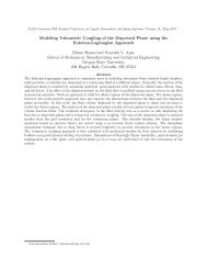
Large-eddy Simulation of Realistic Gas Turbine Combustors

Large-eddy Simulation of Realistic Gas Turbine Combustors
Moin, P. ∗ , & Apte, S. V. †
Center for Integrated Turbulence Simulations
Stanford University, Stanford, CA 94305-3030
http://cits.stanford.edu/
December 1, 2005
Abstract
Large-eddy simulation (LES) is a promising technique for accurate prediction of reacting
multiphase flows in practical gas-turbine combustion chambers involving complex physical phenomena
of turbulent mixing and combustion dynamics. This paper discusses development of
advanced models for liquid fuel atomization, droplet evaporation, droplet deformation & drag,
and turbulent combustion specifically for gas-turbine applications. The non-dissipative, yet robust
numerical scheme for arbitrary shaped unstructured grids developed by Mahesh et al. [1]
is modified to account for density variations due to chemical reactions. A systematic validation
and verification study of the individual spray models and the numerical scheme is performed in
canonical and complex combustor geometries. Finally, a multi-scale, multi-physics, turbulent
reacting flow simulation in a real gas-turbine combustor is performed to assess the predictive
capability of the solver.
∗ Franklin and Caroline Johnson Professor of Mechanical Engineering, Associate Fellow, AIAA, moin@stanford.edu
† Research Associate, Department of Mechanical Engineering. Presently at Oregon State University,
sva@engr.orst.edu
1

1 Introduction
The combustion chambers of gas-turbine based propulsion systems involve complex phenomena
such as atomization of liquid fuel jets, evaporation, collision/coalescence of droplets,
and turbulent mixing of fuel and oxidizer giving rise to spray-flames. Accurate observations
and quantitative measurements of these processes in realistic configurations are difficult and
expensive. Better understanding of these flows for design modifications, improvements, and exploring
fundamental physics demands high-fidelity numerical studies in realistic configurations.
Specifically, good predictive capability for swirling, highly turbulent reacting flows in complex
geometries is necessary.
To date the engineering prediction of such flows in realistic configurations has relied predominantly
on the Reynolds-averaged Navier-Stokes equations (RANS) [2, 3]. In RANS, turbulence
models for the Reynolds stress tensor provide time (or ensemble) -averaged solutions to the
Navier-Stokes equations. Though computationally efficient, RANS-based models for two-phase
reacting flows do not represent the relevant flow quantities accurately even in simple configurations.
LES and direct numerical simulation (DNS) techniques have been shown to give good
predictions of turbulent flows in simple configurations [4]. Recently, Pierce & Moin [5] have
shown the superiority of LES to RANS in accurately predicting turbulent mixing and combustion
dynamics in a coaxial combustor geometry. Kim & Syed [6] and Mongia [7] provide a
detailed overview on the importance and role of LES in designing advanced gas-turbine combustors.
The flowfield inside the combustor is highly swirling, separated and turbulent with
complex features such as mixing of secondary cooling air with hot combustion products. The
spray flame is stabilized by the recirculation bubble created by swirling flow. Multiple, turbulent
jets in cross flow play an important role in scalar mixing; may influence pollutant formation,
and elimination of any ‘hot-spots’ in the combustor exit. LES is considered very attractive in
predicting these flow features and their sensitivity to design modifications. However, presently
LES has largely been used to investigate flows in simple configurations. Our goal is to extend
the LES methodology to realistic geometries involving complex physics of multiphase, reacting
2

flows.
In LES, three-dimensional, unsteady Navier-Stokes equations are spatially filtered, the large
scales are computed directly, and only the effect of unresolved subgrid scales is modeled. The
penalty is increased computational cost. In addition, the numerical algorithms used for LES
must be energy conserving and strictly non-dissipative, as numerical dissipation has been shown
to be detrimental in accurate prediction of turbulent flows [8]. Furthermore, the complex geometry
of practical combustors necessitates use of unstructured grids due to the flexibility they
offer in handling complex configurations as well as significant savings in the number of control
volumes as compared to the body-fitted structured grids.
Recently, Mahesh et. al. [1] have developed a new numerical method with the characteristics
necessary for simultaneously accurate and robust LES on unstructured grids. These competing
ends were achieved by developing a method around the principle of discrete kinetic energy
conservation with no artificial dissipation. Based on this numerical scheme, a parallel, arbitrary
elements, unstructured grid, finite-volume code has been developed specifically to perform
LES of complex combustor geometries. The solver is named after late Charles David Pierce
(1969-2002) who made several lasting contributions to the LES of reacting flows. The original
incompressible formulation by Mahesh et al. [1] is extended to simulate variable density,
low-Mach number flows with integrated models for turbulent combustion and spray dynamics
[9, 10, 11]. In order to trust the numerics and know the limitations of the models used, a
systematic validation and verification study evaluating their predictive capability is of utmost
importance. Detailed experiments independently addressing droplet dispersion, droplet evaporation,
breakup, and turbulent combustion (with gaseous fuel) have been performed, however,
experiments involving multiphase reacting flows in simplified combustors are needed to further
advance the models for spray dynamics and turbulent combustion.
In the following sections, the mathematical formulation for gas and liquid phases, advanced
subgrid models for droplet breakup, evaporation, deformation, and drag are described. Results
from numerous validation studies performed are reported. Ongoing efforts to further develop
advanced physical models and numerical algorithms for improved speedup are summarized.
3

2 Mathematical Formulation
We solve the variable density, low-Mach number, Navier-Stokes equations for the gas-phase.
The formulation is based on flamelet progress-variable (FPV) approach developed by Pierce
& Moin [5] for LES of non-premixed, turbulent combustion.
The liquid phase is treated in
the Lagrangian framework with efficient particle tracking scheme on unstructured grids, which
allows simulation of millions of independent droplet trajectories. A summary of the filtered
Eulerian/Lagrangian equations and subgrid models for unclosed terms and droplet dynamics is
given below.
2.1 Filtered LES Equations for Gas-Phase
The gas phase continuity, scalar, and momentum equations are,
∂ ( ρ g ũ j
)
∂x j
= − ∂ρ g
∂t + Ṡm (1)
( )
∂ ρ g ˜Z
∂t
( )
∂ ρ g ˜C
∂t
∂ ( ρ g ũ i
)
∂t
+
+
)
(
∂
(ρ g ˜Zũj
= ∂ ∂
ρ
∂x j ∂x g ˜α ˜Z
)
Z − ∂q Zj
+
j ∂x j ∂x ṠZ (2)
j
)
(
∂
(ρ g ˜Cũj
= ∂ ∂
ρ
∂x j ∂x g ˜α ˜C
)
C − ∂q Cj
+ ˙ω C (3)
j ∂x j ∂x j
+ ∂ ( ρ g ũ i ũ j
)
∂x j
= − ∂p + ∂(2µ ˜S ij )
− ∂q ij
+
∂x i ∂x j ∂x Ṡi (4)
j
where
˜S ij = 1 ( ∂ũi
+ ∂ũ )
j
2 ∂u j ∂u i
− 1 3 δ ∂ũ k
ij . (5)
∂x k
Here ρ g is the gas-phase density, u j the velocity vector, p the pressure, µ the dynamic
viscosity, δ ij the Kronecker symbol, Z the mixture fraction, C the progress variable, α Z and α C
the scalar diffusivities, and ˙ω C the source term due to chemical reactions. The additional term
4

in the continuity, Ṡ m , mixture fraction, Ṡ Z , and momentum equations, Ṡ i , are the interphase
mass and momentum transport terms. The unclosed transport terms in the momentum and
scalar equations are grouped into the residual stress, q ij , and residual scalar fluxes, q Zj , q Cj .
The filtering operation is denoted by an overbar and Favre (density-weighted) filtering by tilde.
The choice of the progress variable depends on the flow conditions and chemistry. Typically,
mass fractions of major product species is a good indicator of the forward ‘progress’ of the
reaction.
2.2 Presumed P DF approach
Following the FPV appraoch [5], the chemistry is incorporated in the form of a steady-state
one-dimensional flamelet model. Due to the presence of the liquid phase, the transport equation
for the mixture fraction (defined based on the fuel vapor) has a source term (Eq. 2). In addition,
the heat of droplet vaporization is taken from the gas-phase causing evaporative cooling of the
surrounding gas. This gives rise to a sink term in the energy equation. The evaporative cooling
effect is accounted for during the generation of the flamelet tables by computing an effective
gaseous fuel temperature, T fuel,g = T fuel,l − L vap /C pl , where subscript l stands for liquid, L vap
is the latent heat of vaporization, and C pl the specific heat of liquid fuel, and T fuel,l the inlet
liquid fuel temperature. This effective gaseous fuel temperature is used as boundary condition in
solving the flamelet equations. By assuming adiabatic walls and unity Lewis number, the energy
and mixture fraction equations have the same boundary conditions and are linearly dependent.
The energy conservation equation is not solved in this formulation.
The subgrid fluctuations in the mixture fraction and progress variable, filtered combustion
variables are obtained by integrating chemical state relationships over the joint P DF of Z and
C. As an example, the filtered chemical source term of the progress variable is given as,
∫
˙ω C =
˙ω C (Z, C) ˜P (Z, C)dZdC. (6)
The joint subgrid P DF is modeled by writing, ˜P (Z, C) = ˜P (C|Z) ˜P (Z). Here, ˜P (Z) is modeled
5

y the presumed beta subgrid P DF and the conditional P DF , ˜P (C|Z) is modeled as a delta
function according to Pierce & Moin [5]. In the present two-phase flow application, the mixture
fraction equation (Eq. 2) consists of a source term due to the evaporation of liquid fuel. By
assuming a beta P DF for ˜P (Z) we implicitly assume that the time-scale of evaporation is small
compared to the scalar mixing time-scale. More advanced micro-mixing models accounting for
spray-chemistry interactions are necessary [12] to better represent the filtered source terms in the
continuity and mixture-fraction equations. Following these assumptions, the flamelet library is
computed and subgrid P DF integrals are evaluated to generate lookup tables to provide filtered
variables as:
ỹ i = ỹ i ( ˜Z, ˜Z ′′ 2
, ˜C), ˜T = ˜T ( ˜Z, ˜Z ′′ 2
, ˜C), ρ g = ρ g ( ˜Z, ˜Z ′′ 2
, ˜C), etc. (7)
where ˜Z ′′ 2
is the mixture fraction variance, ỹ i the species mass fractions, and ˜T the temperature.
Similar expressions are obtained for dynamic viscosity, molecular diffusivities, and other
properties required in the computation.
2.3 Subgrid Scale Models
The dynamic Smagorinsky model by Moin et al. [13] is used to close the subgrid terms as
demonstrated by Pierce & Moin [14]. The unclosed terms in Eqs. (2-4) are modeled using the
eddy-viscosity assumption. The eddy viscosity, eddy diffusivities, and subfilter variance of the
mixture fraction are evaluated as:
µ t = C µ ρ g ∆ 2 |˜S|, ρ g α t = C α ρ g ∆ 2 |˜S|, ρ g
˜Z ′′ 2
= C ˜Zρ g ∆ 2 | ▽ ˜Z| 2 (8)
where |˜S| =
√
˜Sij ˜Sij . The coefficients C µ , C α , and C ˜Z
are evaluated dynamically [14].
6

2.4 Liquid-Phase Equations
The droplet motion is simulated using the Basset-Boussinesq-Oseen (BBO) equations [15]. It
is assumed that the density of the droplet is much larger than that of the fluid (ρ p /ρ g ∼ 10 3 ),
droplet-size is small compared to the turbulence integral length scale, and that the effect of
shear on droplet motion is negligible. The high value of density ratio implies that the Basset
force and the added mass term are small and are therefore neglected. Under these assumptions,
the Lagrangian equations governing the droplet motions become
du p
dt
dx p
dt
= u p , (9)
(
= D pdrop (u − u p ) + 1 − ρ )
g
g (10)
ρ p
where x p is the position of the droplet centroid, u p the droplet velocity components, u the gasphase
velocities interpolated to the droplet location, ρ p & ρ g the droplet and gas-phase densities,
and g the gravitational acceleration. The drag force on a droplet is modeled by drag coefficient,
C d , based on a solid particle with modifications due to internal circulation and deformation,
D psolid = 3 4 C ρ g |u g − u p |
d
(11)
ρ p d p
where C d is obtained from the nonlinear correlation [15]
C d = 24 ( )
1 + aRe
b
Re
p . (12)
Here Re p = d p |u g − u p |/µ g is the particle Reynolds number. The above correlation is valid for
Re p ≤ 800. The constants a = 0.15, b = 0.687 yield the drag within 5% from the standard drag
curve. The above expression for solid body drag is modified to account for droplet deformation
and internal circulation as given below.
In LES of droplet-laden flows, the droplets are presumed to be subgrid, and the droplet-size
is smaller than the filter-width used. The gas-phase velocity field required in Eq. (10) is the total
7

(unfiltered) velocity, however, only the filtered velocity field is computed in Eqs. (4). The direct
effect of unresolved velocity fluctuations on droplet trajectories depends on the droplet relaxation
time-scale, and the subgrid kinetic energy. Pozorski et al. [16] performed a systematic study
of the direct effect of subgrid scale velocity on particle motion for forced isotropic turbulence.
It was shown that, in poorly resolved regions, where the subgrid kinetic energy is more than
30%, the effect on droplet motion is more pronounced. A stochastic model reconstructing the
subgrid-scale velocity in a statistical sense was developed [16]. In the present work, we neglect
this direct effect of subgrid scale velocity on the droplet motion. However, note that the particles
do feel the subgrid scales through the subgrid model that affects the resolved velocity field. For
swirling, separated flows with the subgrid scale energy content much smaller than the resolved
scales, the direct effect was shown to be small [9].
2.4.1 Deformation and drag models
The drag law for spherical, solid objects (Eq. 11) needs modifications when applied to liquid
droplets in a turbulent flow. Droplet deformation and internal circulation may affect the drag
force significantly. In order to quantify the effect of droplet deformation on drag, Helenbrook &
Edwards [17] performed detailed resolved simulations of axisymmetric liquid drops in uniform
gaseous stream. Based on their computations for a range of density and viscosity ratios, range
of Weber (W e), Ohnesorge (Oh), and Reynolds numbers (Re), a correlation was developed that
provides the amount of droplet deformation in the form of ellipticity, E, which is defined as the
ratio of the height to width of the drop,
√
E = 1 − 0.11W e 0.82 ρp µ g
+ 0.013 Oh −0.55 W e 1.1 (13)
ρ g µ l
where µ l , µ g are the viscosities, and ρ p , ρ g the densities of the liquid and gas-phase, respectively.
The non-dimensional Weber and Ohnesorge numbers are defined as, W e = ρ g U 2 d p /σ and
Oh = µ l / √ ρ p σd p , where U is the relative velocity between the gas and liquid, d p the diameter
of the droplet, and σ the surface tension. Accordingly, E < 1 indicates that the drops have
8

more width than height with deformation in a direction perpendicular to the relative velocity.
These shapes are called oblate shapes. Similarly, E > 1 gives elongation in the direction of the
relative velocity giving rise to prolate shapes. E = 1 implies spherical shapes.
The effect of droplet deformation is reflected in the drag force. This effect is modeled by
using an effective equatorial droplet diameter, d ∗ p = d p E −1/3 . The particle Reynolds number is
also modified, Re ∗ p = Re p E −1/3 . This is used in Eqs. (11, 12) to obtain the modified drag [17].
In addition the effect of internal circulation is modeled by changing the drag on a solid sphere
as
( )
D pdrop 2 + 3µl /µ g (1
=
− 0.03(µg /µ l )Re 0.65 )
p
D psolid 3 + 3µ l /µ g
(14)
2.4.2 Stochastic model for secondary breakup
Performing simulations of primary atomization where one tracks the liquid-gas interface in realistic
combustor geometries is computationally intensive. The current state-of-the art is to compute
the atomization process using subgrid, secondary breakup models based on point-particle
approximation. Emphasis is placed on obtaining the correct spray evolution characteristics such
as liquid mass flux, spray angle, and droplet size distribution. The liquid jet/sheet is approximated
by large drops with size equal to the nozzle diameter. The effect of high mass-loading
on the gas-phase momentum transport is captured through two-way coupling between the two
phases.
A stochastic spray breakup model capable of generating a broad range of droplet sizes at
high Weber numbers has been developed [10]. In this model, the characteristic radius of droplets
is assumed to be a time-dependent stochastic variable with a given initial size-distribution. The
breakup of parent drops into secondary droplets is viewed as the temporal and spatial evolution
of this distribution function around the parent-droplet size according to the Fokker-Planck (FP)
differential equation:
∂T (x, t)
∂t
∂T (x, t)
+ ν(ξ) = 1 ∂x 2 ν(ξ2 ) ∂2 T (x, t)
∂x 2 . (15)
9

where the breakup frequency (ν) and time (t) are introduced. Here, T (x, t) is the distribution
function for x = log(r p ), and r p is the droplet radius. Breakup occurs when t > t breakup = 1/ν.
This distribution function follows a certain long-time behavior, which is characterized by the
dominant mechanism of breakup. The value of the breakup frequency and the critical radius
of breakup are obtained by the balance between the aerodynamic and surface tension forces.
The secondary droplets are sampled from the analytical solution of Eq. (15) corresponding to
the breakup time-scale. The parameters encountered in the FP equation (〈ξ〉 and 〈 ξ 2〉 ) are
computed by relating them to the local Weber number for the parent drop, thereby accounting
for the capillary forces and turbulent properties [10]. As new droplets are formed, parent droplets
are destroyed and Lagrangian tracking in the physical space is continued till further breakup
events.
2.4.3 Evaporation model
Typical spray simulations do not resolve the temperature and species gradients around each
droplet to compute the rate of evaporation. Instead, evaporation rates are estimated based on
quasi-steady analysis of a single isolated drop in a quiescent environment [18, 19]. Multiplicative
factors are then applied to consider the convective and internal circulation effects. We model
the droplet evaporation based on a ‘uniform-state’ model. The Lagrangian equations governing
particle mass and heat transfer processes are well summarized by Oefelein [20] and are described
here in brief.
d
dt (m p) = −ṁ p (16)
m p C pl
d
dt (T p) = h p πd 2 p (T g − T p ) − ṁ p ∆h v (17)
where ∆h v is the latent heat of vaporization, m p mass of the droplet, T p temperature of the
droplet, and C pl the specific heat of liquid. The diameter of the droplet is obtained from its
10

mass, d p = (6m p /πρ p ) 1/3 . The effective heat-transfer coefficient, h p is defined as,
( ) dT
h p = k s / (T g − T s ) (18)
dr
sg
where k s is the effective conductivity of the surrounding gas at the droplet surface. The subscript
‘s’ stands for the surface of the droplet. The expression for ṁ p and solution to Eqs. (16,17)
in quiescent medium are obtained by defining Spalding mass and heat transfer numbers and
making use of the Clausius-Clapeyron’s equilibrium vapor-pressure relationship [18]. In addition,
convective correction factors are applied to obtain spray evaporation rates at high Reynolds
numbers [20].
2.4.4 Hybrid particle-parcel technique for spray simulations
Performing spray breakup computations using Lagrangian tracking of each individual droplet
gives rise to a large number of droplets (≈ 20-50 million) in localized regions very close to
the injector. Simulating all droplet trajectories gives severe load-imbalance due to presence of
droplets on only a few processors. On the other hand, correct representation of the fuel vapor
distribution obtained from droplet evaporation is necessary to capture the dynamics of spray
flames. We have developed a hybrid particle-parcel scheme to effectively reduce the number of
particles tracked and yet represent the overall spray evolution properly [10].
A parcel or computational particle represents a group of droplets, N par , with similar characteristics
(diameter, velocity, temperature). The basic idea behind the hybrid-approach is as
follows. At every time step, droplets of the size of the spray nozzle are injected based on the fuel
mass flow rate. New particles added to the computational domain are pure drops (N par = 1).
These drops are tracked by Lagrangian particle tracking and undergo breakup according to the
stochastic model creating new droplets of smaller size. As the local droplet number density
exceeds a prescribed threshold, all droplets in that control volume are collected and grouped
into bins corresponding to their size and other properties such as velocity, temperature etc. The
droplets in bins are then used to form a parcel by conserving mass, momentum and energy. The
11

properties of the parcel are obtained by mass-weighted averaging from individual droplets in the
bin. The number of parcels created would depend on the number of bins and the threshold value
used to sample them. A parcel thus created then undergoes breakup according to the above
stochastic sub-grid model, however, does not create new parcels. On the other hand, N par is
increased and the diameter is decreased by mass-conservation.
This strategy effectively reduces the total number of computational particles in the domain.
Regions of low number densities are captured by individual droplet trajectories, giving a more
accurate spray representation.
2.5 Interphase Exchange Terms
The source terms in the gas-phase continuity, mixture-fraction, and momentum equations are
obtained from the equations governing droplet dynamics
(Eqs. 10,16). For each droplet the
source terms are interpolated from the particle position (x p ) to the centroid of the grid control
volume using an interpolation operator. The source terms in the continuity and mixture fraction
equations are identical as they represent conservation of mass of fuel vapor. The expressions for
source terms are:
Ṡ m (x) = ṠZ(x) = − 1 ∑
G σ (x, x p ) d V cv dt (m p) (19)
k
Ṡ i (x) = − 1 ∑
G σ (x, x p ) d ) (m p u k p
V cv dt i
(20)
k
where the summation is over all droplets (k), V cv is the volume of the grid cell in which the
droplet lies, and the function G σ is the interpolation operator given as
G σ (x, x p ) =
[ ∑ 3
( ) 2
]
1
(σ √ 2π) exp i=1 xi − x pi
−
3 2σ 2 . (21)
where σ is proportional to the grid size in which the droplet lies. For each droplet, the conservation
constraint, ∫ V cv
G σ (x, x p )dV = 1, is imposed by normalizing the interpolation operator.
12

3 Numerical Method
A co-located, finite-volume, energy-conserving numerical scheme on unstructured grids has been
developed by Mahesh et al. [1] to solve the gas-phase incompressible flow equations. The velocity
and pressure are stored at the centroids of the control volumes. The cell-centered velocities are
advanced in a predictor step such that the kinetic energy is conserved. The predicted velocities
are interpolated to the faces and then projected. Projection yields the pressure potential at
the cell-centers, and its gradient is used to correct the cell and face-normal velocities. A novel
discretization scheme for the pressure gradient was developed by Mahesh et al. [1] to provide
robustness without numerical dissipation on grids with rapidly varying elements. This algorithm
was found to be imperative to perform LES at high Reynolds numbers in realistic combustor
geometries.
This formulation has been shown to provide very good results for both simple and complex
geometries [1] and is extended to variable density, low Mach number equations to compute turbulent
reacting flows [11]. In addition, for two-phase flows the particle centroids are tracked using
the Lagrangian framework. The particle equations are integrated using third-order Runge-Kutta
schemes. After obtaining the new particle positions, the particles are relocated, particles that
cross interprocessor boundaries are duly transferred, boundary conditions on particles crossing
boundaries are applied, source terms in the gas-phase equation are computed, and the computation
is further advanced. Solving these Lagrangian equations thus requires addressing the
following key issues: (i) efficient search for locations of particles on an unstructured grid, (ii)
interpolation of gas-phase properties to the particle location for arbitrarily shaped control volumes,
(iii) inter-processor particle transfer. An efficient Lagrangian framework was developed
which allows tracking millions of particle trajectories on unstructured grids [9].
4 Results: Validation Studies
A systematic approach is taken to perform validation studies to assess the predictive capability
of the numerical scheme used as well as different physical models described in section 2.
13

The basic idea is to isolate physical phenomena of droplet/particle motion, droplet breakup,
evaporation, and turbulent combustion and simulate them in canonical problems where detailed
description of the boundary conditions and in-depth experimental data are available. This also
allows development and testing of new models and numerical schemes for flows of interest.
The following cases with well specified boundary conditions have been simulated: 1) swirling,
particle-laden flow in a co-annular jet (experiments by Sommerfeld & Qiu [21]), 2) evaporating
droplets in a turbulent flow (experiments by Sommerfeld & Qiu [22]), 3) high-speed liquid jet
atomization in a cylindrical chamber (experiments of Hiroyasu & Kudota [23]), and 4) turbulent
reacting flow with gaseous fuel (experiments by Spadaccini et. al. [24]). After verifying
the predictive capability of the numerical scheme and models used for these flows, the following
simulations in realistic combustor geometries were performed: 5) non-reacting, gaseous flow in a
PW test rig representative of realistic conditions, 6) non-reacting flows in a real PW combustor,
7) liquid-spray patternation experiments of the PW injector, and 8) a multiphase, multiphysics
simulation of reacting flow in real PW combustor.
In this work, emphasis is placed on validation of spray dynamics and details of cases 1-3, and
7-8 are presented next. The numerical results of case 4 and cases 5-6 have been well documented
by Mahesh et al. [1, 11], respectively and are not repeated here.
4.1 Validation of Eulerian-Lagrangian Formulation
The Eulerian-Lagrangian formulation on unstructured grids is validated by simulating a swirling,
particle-laden cold flow in a coaxial geometry corresponding to the experiments of Sommerfeld
& Qiu [21]. This flow configuration was chosen because the basic flow features with swirling
jets and recirculation bubbles resemble those inside a gas-turbine combustor. In addition, the
boundary conditions are very well specified along with detailed statistics for the gas and particle
phase at various locations making it an important validation case.
Figure (1) shows a slice through the axisymmetric flow configuration which consists of a
central core (primary) and annular (secondary) jets discharging into a cylindrical test section
14

with sudden expansion. The primary jet has a radius of 16 mm and is laden with glass beads
with a mean number diameter (D 10 ) of 45 µm distributed between 10 and 120 µm obtained
by matching an upper-limit log-normal distribution with the experimental measurements. The
secondary annular jet has a swirling azimuthal velocity and extends over the radial interval of
19-32 mm. The outer radius of the annulus (R) is 32 mm, the whole test-section is 960 mm
long, is oriented vertically with gravity acting in the direction of the flow and is connected to
a stagnation chamber of length 640 mm and radius 288 mm. The computational domain is
divided in ∼ 1.6 × 10 6 hexahedral volumes and approximately 96 grid points are used in the
azimuthal direction. The Reynolds number of the primary jet is 26200, the particle loading ratio
of 0.034 is too small to have dense clusters of particles, and the particle-particle interactions are
neglected.
Figure (1) also shows the instantaneous contours of normalized axial velocity in the symmetry
plane (z = 0) along with particle locations superimposed on the turbulent velocity field.
The size of the circles scales with the actual diameter of the particles. The velocity field is
normalized by the average inlet velocity of 12.82m/s. The expansion of the swirling jet, central
and secondary recirculation regions are clearly visible. The gas-phase inflow conditions are generated
by simulating a periodic pipe and annulus with the desired mass flowrates and Reynolds
numbers. Each particle injected into the computational domain is simulated giving around 1.1
million particles at stationary state. Close to the entrance of the test-section at x/R = 0, particles
are concentrated in the central core region. Particles are injected with the same velocities
as the gas-phase at the inlet, however, majority of them do not follow the rapid expansion and
deceleration of the gas jets. These particles are convected downstream and spread in the radial
and azimuthal directions, some of them are trapped in the central recirculation region. Particles
tend to have higher velocities in the core region, penetrate the central recirculation region,
move against the gas-phase flow till they are decelerated to zero axial velocity. These particles
then change their directions, and are thrown radially outwards by the centrifugal action.
Heavier particles penetrate the recirculation bubble the most because of their larger inertia.
The basic features of particle-laden, swirling flows, such as the recirculation bubble length, the
15

eattachment points, the trajectories of different particle sizes are accurately captured [9].
It is important to note that accurate prediction of these flow features plays an important
role in investigating swirling, turbulent flows in gas-turbine combustors. Figure (2) shows comparison
with the experimental data of azimuthally averaged particle-phase mean and rms axial,
swirl, and radial velocity at different cross-sections. Also shown are the mean and rms particle
diameter distributions indicating good agreement. Important particle-dispersion characteristics
are obtained from this simulation to further investigate swirling, particle-laden flows [9].
It
is also confirmed that LES together with the point-particle approach for dispersed phase can
accurately predict swirling, separated flows for dilute-particle loadings.
4.2 Validation of evaporation model and variable density formulation
In order to validate the evaporation model and the variable density formulation, simulation of a
coaxial non-swirling jet has been performed following the configuration used in the experiments
of Sommerfeld & Qiu [22]. This experiment also is well documented with specified boundary
conditions for both phases. For the liquid phase the inlet droplet size distribution and their
correlation with droplet velocity are well-defined.
The gas-phase temperatures are not high
enough to produce spray flames.
This isolates the droplet evaporation problem from spray
breakup and combustion, and makes it suitable to validate the evaporation models.
Figure (3) shows a snapshot of fuel mass fraction contours superimposed by scatter plot of
Isopropyl alcohol droplets in the symmetry plane (z = 0). Hot air at 373K is injected through
the annulus and liquid droplets at 313K are injected along the central wall region according to
the measured size-velocity correlations at x = 3 mm downstream of the wall [22]. The grid used
consists of 1.5M hexahedral cells and around 0.75M particles are present in the computational
domain at statistically stationary state. The droplets are injected near the inlet circular wall
of cross-sectional radius R = 20 mm.
The droplet velocity-size correlation depicts a conical
spray with a spray angle of around 60 0 . The Reynolds number at inlet annulus is 21164 and
the gas-phase inflow velocity is obtained by pre-computing a periodic annulus flow at same
Reynolds number and mass-flow rate and storing instantaneous velocity profiles over 10 flow
16

through times. A convective boundary condition is used at the exit plane. The combustor walls
exhibit some heat losses as measured by the experiments, however, these are assumed small and
adiabatic conditions are applied.
Figure (4) shows the radial variations of the mean and rms droplet velocity, and the mean and
rms of droplet diameter compared to the experimental data. At x/R = 0 and x/R = 0.786 the
profiles of the mean droplet axial velocity show two peaks associated to the hollow-cone spray.
The droplet mean diameter shows a typical result corresponding to a hollow cone atomizer,
where smaller droplets are found in the core region and larger droplets near the edge of the
spray. Away from the injector, the spreading of the spray is hindered by the annular air-jets,
the droplet mean diameter becomes more uniform over the cross-section and slowly decreases
in the downstream direction because of evaporation.
The axial mass-flux (not shown) also
decreases toward the exit due to evaporation and is well captured by the present simulation.
To further validated the the low-Mach number, variable density formulation on unstructured
grids at higher density ratios, a non-premixed methane-air flame in a coaxial combustor has been
simulated. Details of this simulation have been addressed by Mahesh et al. [11] and are not
presented here.
4.3 Validation of stochastic breakup model
To validate the stochastic breakup model together with the hybrid algorithm, a standard test
case for high-speed liquid atomization in a cylindrical chamber is simulated. The computational
domain is a closed cylindrical chamber of length 13.8 cm and diameter 5.6 cm, following the
experimental setup by Hiroyasu and Kudota [23]. Liquid jet is injected through a single-hole
nozzle into this constant pressure, room-temperature nitrogen chamber.
Since the chamber
temperature is low, evaporation of the liquid fuel is negligible. The initial droplet diameter
is 300 µm corresponding to the nozzle size. The number of droplets injected per iteration is
determined based on the droplet diameter and time-step by keeping the mass flow rate constant.
The time step used in this simulation is 15 µs and a uniform grid of 100×65×65 cells is found to
capture the spray dynamics accurately. This configuration was chosen because of its simplicity
17

and several different models have been calibrated against this experiment. In addition, the gasphase
is initially at rest, and any flow generated is through the momentum transfer from the
liquid to the gas-phase allowing us to investigate the two-way coupling effects. The gas-phase
flow generated alters the relative velocity between the droplets and the flow, changes the breakup
time-scale and plays an important role in capturing the spray penetration depth accurately.
The simulation was carried out at three different chamber pressures using the hybrid approach
outlined in section 2.4.4. Figure (5) shows the time evolution of liquid spray at 1.1MPa.
The region close to the injector mostly consists of large unbroken drops along with small, stripped
droplets. The ligament-like liquid structures deflected outward are clearly visible. Comparison
of penetration depth to experimental data at different chamber pressures obtained from the hybrid
approach is shown in Fig. (6). Other spray characteristics such as liquid core length, spray
angle, and the Sauter mean diameter (SMD) are also in good agreement with the experimental
data [10].
4.4 Validation of spray patternation study for realistic PW injector
The stochastic model along with the hybrid particle-parcel approach are used to compare the
prediction of spray patternation characteristics for a realistic PW injector with the experimental
data. The experimental data set [25] was obtained by mounting the actual injector in a cylindrical
plenum through which gas with prescribed mass-flow rate was injected. Figure (7a) shows a
cut through the symmetry plane (z = 0) of the computational domain along with the mesh and
boundary conditions used. For this case, 3.2M grid points are used with high resolution near
the injector. The domain decomposition is based on the optimal performance of the Eulerian
gas-phase solver on 96 processors. Air from the inlet plenum goes through the central core,
guide, and outer swirlers to create multiple swirling jets. All the passages through the swirler
are computed. Also shown are the instantaneous axial velocity contours superimposed by the
droplet locations (Fig. 7b). The swirling air jet from the core swirler enters the dump region
and forms a recirculation zone. Jets from guide and outer swirlers interact with the core flow. A
complex vortex break down phenomenon is observed and its accurate prediction is necessary to
18

correctly represent the injector flow. Substantial amount of air is entrained in the radial direction
and the rate of air entrainment is specified based on the experimentally measured values.
Liquid film is injected through the filmer surface which forms an annular ring. In the symmetry
plane this is indicated by two points on the edge of the annular ring (Fig. 7b).
The liquid
mass-flow rate corresponds to certain operating conditions of the gas-turbine engine. Actual
numbers are not listed because of the proprietary nature of the experimental data. However,
comparisons are presented in terms of normalized quantities or percentage errors.
The liquid film at the filmer surface, is approximated by injecting uniform size drops of the
size of the annular ring thickness. These drops are convected downstream by the swirling air
and undergo breakup according to the stochastic model. A large number of droplets are created
in the vicinity of the injector due to breakup as shown in Fig. (7b). With the hybrid approach,
the total number of computational particles tracked at stationary state is around 3.5M and
includes around 150,000 parcels. Together these represent aproximately 13M droplets. Even
with the hybrid approach, the load-imbalance due to atomization was found to be significant
as only 1/3 rd of the processors had more than 10,000 computational particles. Dynamic loadbalancing
techniques to reduce this computational overhead due to sprays are being investigated
to improve the overall speedup [26].
Figure 8 compares LES predictions to the available experimental data of radial variations of
mean axial and swirl velocity at different axial locations (x = 0.4, x = 1.1, and x = 2.1, where x
is the distance from the injector wall normalized by the reference length scale). The numerical
results are azimuthally averaged. The predictions from our simulation are in close agreement
with the experimental data. Small disagreement at x = 2.1 is partly related to the coarse grid
resolution used away from the injector. It should be noted that the amount of swirl generator
by the injectors determines the size of the recirculation zone. Good agreement of the axial and
swirl velocities indicate that LES with dynamic sgs model can capture the vortex break-down
phenomenon accurately in complex geometries. Also shown are the corresponding predictions
using an in-house k − ɛ model. The unsteady RANS solutions are in agreement with the LES
and experimental data very close to the injector, however, degrade rapidly further away, showing
19

limitations of the turbulence model. Improved predictions using advanced RANS models can
be obtained, however, the superiority of LES is clearly demonstrated. It should be noted that,
any artificial dissipation or inaccurate numerics gives faster decay of the swirl velocities and
incorrect size of the recirculation region, further emphasizing the importance of non-dissipative
numerical schemes for LES.
Figure (9) compares radial variation of liquid mass-flowrates using LES and the stochastic
model to the experimental data. The flow rates are presented as the ratio of the effective to the
integrated flow rate. The effective flow rate is defined as the flow rate the patternator would
record if the fuel flux was uniform at the local value. This normalization inherently carries the
ratio of the total cross-sectional area to the area of the local patternator holes. Also shown
are the predictions made by the k − ɛ model together with the Taylor-Analogy Breakup (TAB)
model [27] commonly used in industry. The LES results are generally in good agreement with
the experiments. Average droplet sizes at two axial location from the injector wall (x = 1.1
and x = 2.1) have been measured using the Malvern line of sight technique. The Sauter mean
diameters averaged over the cross-section at these two axial locations are predicted within 5%
of the experimental values. The present LES with stochastic breakup model predicts a broader
distribution (not shown) as opposed to the one predicted by RANS with TAB model.
The
size distributions also indicate presence of large number of small size droplets compared to
the experiments. This is attributed to the lack of collision/coalescence models in the present
simulation. In addition, the initial droplet size at the injector nozzle is assumed to be a constant,
whereas it may vary depending on the local conditions governing primary atomization. A further
investigation with inclusion of collision models as well as using a size distribution at the inlet
should be performed in order to investigate uncertainties in model predictions.
20

5 Validation of Multi-physics Reacting Flow Simulation
in PW Combustor
A multiscale, multiphysics simulation of turbulent reacting flow in a realistic Pratt & Whitney
combustor has been performed. This includes all the complex models for spray breakup,
evaporation, and turbulent combustion described in section (2.4). Figure (10a) shows a section
through the symmetry plane of the combustor geometry along with contours of temperature.
Also shown are the instantaneous droplet locations in this plane forming a conical spray. The
computational grid consists of 1.9M hybrid elements (hexes, pyramids, and tets) with fine resolution
close to the injector. The grid inside the combustion chamber is hex-dominant to obtain
good numerical accuracy. This simulation is performed on a single (1/18 th ) sector of the full
combustor. The injector is same as the one used in the liquid fuel patternation study described
earlier (section 4.4). The experimental data available for validation includes mass-splits through
different components, temperature profile, and distribution of pollutants, NOx at the measurement
plane.
Liquid fuel (Jet-A) enters the combustion chamber through an annular ring at the injector
exit. This liquid film is approximated by large drops of the size of the injector annulus. These
drops are convected by the surrounding hot air, they break, evaporate, and the fuel vapor thus
formed mixes with the surrounding air giving a non-premixed spray flame. The flamelet library
for Jet-A fuel at gas-turbine engine operating conditions, is generated by using a surrogate fuel
(80% n-Decane and 20% 1-2-4 tri-methyl-benzene) chemistry which closely follows the chemical
kinetics and reaction rates of the Jet-A fuel. Around 1000 elementary reactions among 100
chemical species are used to generate these tables.
The chemical kinetics of surrogate fuel
compared to the original fuel chemistry in terms of prediction of pollutants in laminar flames
showed good agreement [28]. The progress variable for this simulation represents the summation
of mass fractions of CO 2 and H 2 O.
Figure (10b) shows instantaneous snapshots of normalized temperature at various crosssections
from the injector nozzle. High temperatures in the combustion chamber are reduced
21

y cold air influx through the dilution holes. This reduces the exit temperature considerably.
The prediction of mass-splits through different components was shown to be within 5% of the
experimental data for the cold and reacting flow simulations [1, 11] and are not repeated here.
In addition, the average temperature in the measurement plane is within 2% of the experimental
data. The comparison of the radial variation of the mean temperature is shown in Fig. (11) and
was obtained by taking azimuthal average over the sector. This represents our first attempt to
perform such large-scale simulations in realistic configurations and the results give considerable
insight into the combustor spray-flame dynamics.
This computation has been performed on 80 processors of ASC Frost (IBM SP3) and involved
around 0.6M computational particles. It takes around 25-30 CPU-days on ASC Frost to obtain
statistics over 40 time units (3-4 flow through times) starting from a statistically stationary
solution. Significant advances in numerical algorithms resulting in efficient speedup of the solver
are underway [26]. These new algorithms are expected to make possible such a multiphysics,
multiphase computation of the full 18 injector combustor on 100M control volumes within 120-
150 CPU-hrs on the full ASC Frost machine (1024 processors). In addition, advanced models for
prediction of pollutants and NOx are being developed and applied to compute their distributions
within the combustion chamber. A variety of flow conditions including cruise, high power, takeoff
etc. are also being simulated for multiple sectors of the combustor.
6 Summary & Future Work
A non-dissipative, energy-conserving numerical solver for arbitrary-shaped unstructured grids
is developed to simulate multiphase, multiscale turbulent reacting flows in realistic gas-turbine
combustors. This numerical tool solves low-Mach number, variable density flow equations for
the gas-phase. Advanced models to capture atomization & droplet breakup, droplet evaporation,
droplet deformation & drag, and turbulent combustion have been developed to simulate
complex multiphase reacting flows. In this paper, we emphasize the necessity of performing
detailed validation and verification studies to assess the predictive capability of the numerical
22

solver as well as the models used. A series of validation cases in canonical configurations were
selected to systematically evaluate each component of the numerical solver: particle-laden flows,
evaporating droplets, gas-phase combustion, and droplet breakup. Results predicted show good
agreement with the experimental data. Having verified the good predictive capability, a spray
patternation study for PW injector and a multiphysics, multiscale simulation of reacting flow in
one sector of the PW combustor were performed to give encouraging results and considerable
insight into the unsteady flow development inside the combustor.
Advanced numerical schemes handling primary atomization and liquid sheet breakup [29],
finite-size effects of the droplets in the dense-spray regime [30], models for liquid-film formation
[31], droplet dispersion [16], models based on concepts of micro-mixing for droplet flame
interactions, advanced combustion models for premixed/partially premixed turbulent flames,
soot and pollutant formation, and radiation are being developed. In addition, a highly accurate
numerical scheme capturing acoustic waves without the stringent acoustic CFL-restriction in
compressible flows has been developed to investigate combustion instabilities [32]. An extensive
effort is ongoing to make this tool efficient (by using multigrid solvers, dynamic load-balancing
techniques), modular, user-friendly and capable of solving relevant industrial problems with
quick turn around time to suit the demands of combustor design cycle in aircraft industry.
7 Acknowledgement
Support for this work was provided by the United States Department of Energy under the
Accelerated Strategic Computing (ASC) program and NASA’s UEET program. The computations
were performed on Blue Horizon at San Diego supercomputing center and ASC Frost at
Lawrence Livermore National Laboratory. We are grateful to the Pratt & Whitney’s combustor
group for providing important data for validation. The help provided by Prof. Krishnan Mahesh
(University of Minnesota), Drs. Gianluca Iaccarino, Frank Ham, Prof. Heinz Pitsch (Stanford
University), and Prof. George Constantinescu (University of Iowa) is highly appreciated.
23

References
[1] Mahesh, K., Constantinescu, G., and Moin, P., “A New Time-Accurate Finite-
Volume Fractional-Step Algorithm for Prediction of Turbulent Flows on Unstructured
Hybrid Meshes,” J. Comput. Phys., Vol. 197, 2004, pp. 215–240.
[2] Malecki, R.E., Rhie, C.M., Colket, M.B., Madabhushi, R.K., McKinney,
R.G., Ouyang, H., and Syed, S.A., “Application of an Advanced CFD-Based Analysis
System to the PW6000 Combustor to Optimize Exit Temperature Distribution -
Part I: Description and Validation of the Analysis Tool,” ASME Turbo Expo, Paper No.
2001-GT-0062, 2001.
[3] Brankovic, A., McKinney, R.G., Ouyang, H., Porter, L., Kenndy, J., Madabhushi,
R., and Colket, M., “Comparison of Measurements and Predictions of Flow
in a Gas Turbine Engine Fuel Nozzle,” AIAA Paper No. 2001-0331, 2000.
[4] Moin, P., and Mahesh, K., “Direct Numerical Simulation: a Tool in Turbulence
Research,” Ann. Rev. Fluid Mech., Vol. 30, 1998, pp. 539–578.
[5] Pierce, C.D., and Moin, P., “Progress-Variable Approach for Large-eddy Simulation
of Turbulent Non-Premixed Combustion,” J. Fluid Mech., Vol. 504, 2004, pp. 73–97.
[6] Kim, W.-W., and Syed, S., “Large-eddy Simulation Needs for Gas-Turbine Combustor
Design,” AIAA Paper No.2004-0331, AIAA Aerospace Sciences Meeting, Reno, NV,
2004.
[7] Mongia, H.. “Recent Advances in the Development of Combustor Design Tools,” AIAA
Paper No. 2003-4495.
[8] Mittal, R., and Moin, P., “Suitability of Upwind-Biased Finite Difference Schemes
For Large-eddy Simulations of Turbulence Flows,” AIAA J., Vol. 35, 1997, pp. 1415–
1417.
24

[9] Apte, S. V., Mahesh, K., Moin, P., and Oefelein, J.C. “Large-eddy Simulation
of Swirling Particle-Laden Flows in a Coaxial-Jet Combustor,” Int. J. Mult. Flow, Vol.
29, 2003, pp.1311-1331.
[10] Apte, S. V., Gorokhovski, M. and Moin, P., “LES of atomizing spray with stochastic
modeling of secondary breakup,” Int. J. Mult. Flow, Vol. 29, 2003, pp.1503–1522.
[11] Mahesh, K., Constantinescu, G., Apte, S.V., Iaccarino, G., Ham, F., and
Moin, P., “Large-eddy Simulation of Reacting Turbulent Flows in Complex Geometries,”
ASME J. App. Mech., accepted for publication, 2005.
[12] Reveillon, J., and Vervisch, L. “Spray Vaporization in Non-premixed Turbulent
Combustion Modeling: A Single Droplet Model,” Comb. Flame, Vol. 121, 2000, pp.75–
90.
[13] Moin, P., Squires, K., Cabot, W., and Lee, S., “A dynamic subgrid model for
compressible turbulence and scalar transport,” Phy. Fluid A., Vol. 3, 1991, pp.2746–
1757.
[14] Pierce, C.D., and Moin, P., “A Dynamic Model for Subgrid-Scale Variance and
Dissipation Rate of a Conserved Scalar,” Phy. Fluids, Vol.10, 1998, pp.3041–3044.
[15] Crowe, C., Sommerfeld, M., and Tsuji, Y., Multiphase Flows with Droplets and
Particles, CRC Press, Boca Raton, FL, 1998.
[16] Pozorski, J., Apte, S.V., and Raman, V. “Filtered Particle Tracking for Dispersed
Two-Phase Flows,” Proceedings of the Summer Program, Center for Turbulence Research,
Stanford University, 2004, (http://ctr.stanford.edu/).
[17] Helenbrook, B. T., and Edwards, C. F., “Quasi-steady Deformation and Drag of
Uncontaminated Liquid Drops,” Int. J. Multi. Flows., Vol. 28, 2002, pp.1631–1657.
[18] Faeth, G., “Current status of droplet and liquid combustion,” Prog. Energy Combust.
Sci., Vol. 3, 1977, pp.191–224.
[19] Faeth, G., “Evaporation and combustion of sprays,” Prog. Energy Combust. Sci., Vol.
9, 1983, pp.1–76.
25

[20] Oefelein, J. C., “Simulation and analysis of turbulent multiphase combustion processes
at high pressures,” Ph.D. Thesis, The Pennsylvania State University, University
Park, Pa, 1997.
[21] Sommerfeld, M., and Qiu, H.H., “Detailed measurements in a swirling particulate
two -phase flow by a phase - Doppler anemometer,” Int. J. Heat & Fluid Flow, Vol. 12,
No. 1, 1991, pp.20–28.
[22] Sommerfeld, M., and Qiu, H.H., “Experimental studies of spray evaporation in
turbulent flow,” Int. J. Heat & Fluid Flow, Vol. 19, 1998, pp.10–22.
[23] Hiroyasu, M., and Kudota, T., “Fuel droplet size distribution in diesel combustion
chamber,” SAE Tech. Paper: 740715, 1974.
[24] Spadaccini, L.J., Owen, F.K., and Bowman, C.T., “Influence of aerodynamic phenomena
on pollutant formation in combustion (Phase I. Gaseous fuels),” U.S. Environmental
Protection Agency Report EPA-600/2-76-247a, 1976.
[25] McKinney, R., Madabhushi, R.K., and Syed, S., private communication, 2002.
[26] Ham, F., Apte, S.V., Iaccarino, G., Wu, X., Herrmann, M., Constantinescu,
G., Mahesh, K., and Moin, P., “Unstructured LES of Reacting Multiphase Flows
in Realistic Gas-Turbine Combustors,” Annual Research Briefs, Center for Turbulence
Research, Stanford University, 2003, pp. 139–160, (http://ctr.stanford.edu).
[27] O’Rourke, P.J., and Amsden, A. A., “ The TAB method for numerical calculations
of spray droplet breakup,” SAE Technical Paper, No. 87-2089, 1987.
[28] Riesmeier, E, Honnet S, Peters N “Flamelet Modeling of Pollutant Formation in
a Gas Turbine Combustion Chamber Using Detailed Chemistry for a Kerosene Model
Fuel,” ASME J. Engr. Gas Turb. & Power-Tran., Vol. 126, No. (4), 2004, pp.899–905.
[29] Herrmann, M., “A Level-Set/Vortex Sheet Method for Two-Phase Interface Dynamics,”
J. Comp. Phys., Available online, October, 2004.
26

[30] Apte, S.V., Mahesh, K., and Lundgren, T., “A Eulerian-Lagrangian Model to
Simulate Two-Phase Particulate Flows,” Annual Research Briefs, Center for Turbulence
Research, Stanford University, 2003, pp.161–171, (http://ctr.stanford.edu/).
[31] Kim, W.-W, Apte, S.V., Herrmann, M., and Ham, F. “Liquid Film Modeling in
Jet Engine Fuel Injectors,” Proceedings of the Summer Program, Center for Turbulence
Research, Stanford University, 2004, (http://ctr.stanford.edu/).
[32] C. Wall, C. D. Pierce, and P. Moin, “A semi-implicit method for resolution of
acoustic waves in low mach number flows”. J. Comp. Phys., Vol. 181, No. (2), 2002, pp.
545–563.
y/R
3
2
1
0
-1
-2
-3
0 5 10 15
x/R
1.5
1.2
0.8
0.5
0.2
-0.2
-0.5
Figure 1: Snapshot of axial velocity contours superimposed by scatter plot of glass-particles in
particle-laden, swirling flow in a co-axial jet combustor simulating experiment by Sommerfeld &
Qiu [21]. The velocity scale is normalized by average inlet velocity of 12.82m/s.
27

x/R=0.094
3
0.781
1.63
2.66
3.5
4.84
3 x/R=0.094
0.781
1.63
2.66
3.5
4.84
2
2
1
1
0
0 1
0 1
0 1
(a)
0 1
0 1
0 1
0
0 0.5
0 0.5 0 0.5 0 0.5
(b)
0 0.3
0 0.3
0.781
1.63
2.66
3.5
4.84
3 x/R=0.094
0.781
1.63
2.66
3.5
4.84
2
2
1
1
0
0 0.5
0 0.5
3 x/R=0.094 (d)
0 0.5
(c)
0 0.5
0 0.5
0 0.5
0
0 0.3
0 0.3
0 0.3
0 0.3
0 0.3
0 0.3
0.781
1.63
2.66
3.5
4.84
x/R=0.094
3
0.781
1.63
2.66
3.5
4.84
2
2
1
1
0
0 0.5
0 0.5
3 x/R=0.094 (f)
0 0.5
(e)
0 0.5
0 0.5
0 0.5
0
0 0.2
0 0.1
0 0.1
0 0.1
0 0.1
0 0.1
0.781
1.63
2.66
3.5
4.84
3 x/R=0.094
0.781
1.63
2.66
3.5
4.84
2
2
1
1
0
0 50
0 50
0 50
3 x/R=0.094 (h)
(g)
0 50
0 50
0 50
0
0 30
0 20
0 20
0 20
0 20
0 20
Figure 2: Comparison of particle statistics obtained from LES ( ) to experimental data (◦ )
of Sommerfeld & Qiu [21] at different axial locations (x normalized by the reference annulus radius
R = 32mm): (a) mean axial velocity, (b) rms axial velocity, (c) mean radial velocity, (d) rms radial
velocity, (e) mean swirl velocity, (f) rms of swirl velocity, (g) mean diameter (microns), (h) rms
of particle diameter (microns).
28

0.001 0.003 0.006 0.008 0.011 0.013 0.016 0.018 0.021 0.023
Y
2
1
0
Hot Air
Spray
-1
-2
0 5 10
Figure 3: Snapshot of fuel mass fraction superimposed by droplet scatter plot in the symmetry
plane (z = 0) of a co-axial combustor simulating experiment by Sommerfeld & Qiu [22].
X
29

50
X/R = 0.786
X/R = 1.56
X/R = 3.125
X/R = 6.25
X/R = 9.375
X/R = 12.5
(a)
R, mm
0
-50
0 10 20
0 10 20
0 10 20
0 10 20
0 10 20
0 10 20
R, mm
50
0
50
0
(b)
-50
-50
0 2 4
0 2 4 0 2 4 0 2 4 0 2 4
0 2 4
50
(c)
R, mm
0
-50
0 50 100
0 50 100 20 40 60
20 30 40 50 20 30 40
10 20 30 40
50
(d)
R, mm
0
-50
0 20 40
0 20 40
0 20 40 0 10 20 0 10 20
0 10 20
Figure 4: Radial variations of droplet statistics at different axial locations (x normalized by the
core radius R = 20mm) compared to experimental data of Sommerfeld & Qiu [22], LES,
◦ experimental data: a) mean axial velocity (m/s) b) rms of axial velocity, (m/s) c) mean diameter
(microns), and d) rms diameter (microns).
30

0.5
t=0.18 ms
y, cm
0
-0.5
0 0.5 1 1.5 2 2.5
0.5
t=0.38 ms
y, cm
0
-0.5
0 0.5 1 1.5 2 2.5
0.5
t=0.6 ms
y, cm
0
-0.5
0 0.5 1 1.5 2 2.5
x, cm
Figure 5: Time evolution of high speed liquid jet undergoing breakup in a closed cylindrical chamber
at P=1.1MPa.
31

Penetetration Depth, cm
12
9
6
3
LES, 1.1MPa
Exp, 1.1MPa
LES, 3MPa
Exp, 3MPa
LES, 5MPa
Exp, 5MPa
0
0 0.5 1 1.5 2 2.5 3 3.5
Time, ms
Figure 6: Validation of stochastic model with hybrid approach for atomization of high-speed liquid
jet. Prediction of liquid spray penetration depth at different chamber pressures compared with
experimental data by Hiroyasu & Kudota [23].
32

y
6
4
2
0
(a)
inlet
wall
outer swirler
core
swirler
entrainment
outlet
2
1
0
(b)
droplet
injection
-2
guide swirler
-1
-4
wall
entrainment
-2
-6
-5 0 5
x
0 2
x
Figure 7: Snapshot of the symmetry plane (z = 0) of a PW injector: a) the full computational
domain indicating boundary conditions and computational mesh, b) instantaneous droplet locations
in the symmetry plane along with axial velocity contours. x and y are normalized axial and radial
coordinates.
33

300 (a)
200
(b)
Axial Velocity
200
100
0
Swirl Velocity
100
0
-100
-100
-2 -1.5 -1 -0.5 0 0.5 1 1.5 2
-200
-2 -1.5 -1 -0.5 0 0.5 1 1.5 2
Axial Velocity
200
150
100
50
0
-50
(c)
Swirl Velocity
150
100
50
0
-50
-100
(d)
-100
-2 -1.5 -1 -0.5 0 0.5 1 1.5 2
-150
-2 -1.5 -1 -0.5 0 0.5 1 1.5 2
200
(e)
100
(f)
Axial Velocity
100
0
Swirl Velocity
50
0
-50
-100
-2 -1.5 -1 -0.5 0 0.5 1 1.5 2
Normalized Radius
-100
-2 -1.5 -1 -0.5 0 0.5 1 1.5 2
Normalized Radius
Figure 8: Radial variation of normalized mean axial and swirl velocities at different axial locations
for the PW injector patternation study: ◦ experimental data [25], LES, Unsteady RANS
using k − ɛ model: (a-b) x = 0.4, (c-d) x = 1.1, (e-f) x = 2.1. Here x is the normalized distance
from the injector wall.
34

Normalized Axial Mass Flowrate
8
6
4
2
(a)
0
0 0.5 1 1.5 2
Normalized Radius
6
5
4
3
2
1
(b)
0
0 0.5 1 1.5 2
Normalized Radius
Figure 9: Comparison of radial variation of normalized liquid axial mass flux at two axial locations
for the PW injector spray patternation study: Unsteady RANS with TAB model for breakup,
present LES with stochastic breakup model, ◦ — ◦ experimental error bar: a) x = 1.1, b)
x = 2.1 where x is the normalized distance from the injector wall.
35

(a)
(b)
Figure 10: Instantaneous snapshot of temperature in the Pratt & Whitney combustor obtained from
LES: a) symmetry plane with superimposed droplet locations, b) temperature contours at different
cross-sections from the injector nozzle, the last plane represents the temperature measurement
plane.
36