Observer/Kalman-Filter Time-Varying System Identification - AIAA
Observer/Kalman-Filter Time-Varying System Identification - AIAA
Observer/Kalman-Filter Time-Varying System Identification - AIAA
Create successful ePaper yourself
Turn your PDF publications into a flip-book with our unique Google optimized e-Paper software.
892 MAJJI, JUANG, AND JUNKINS<br />
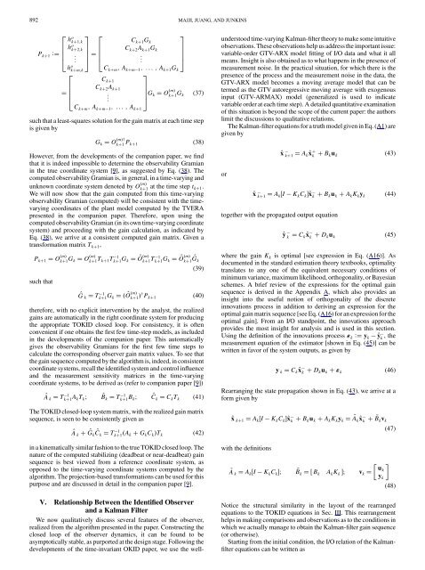
P k 1<br />
:<br />
2<br />
h o 3 2<br />
3<br />
k 1;k<br />
C k 1 G k<br />
h o k 2;k<br />
C k 2 A k 1 G k<br />
6 . 7 6<br />
.<br />
7<br />
4 . 5 4<br />
.<br />
5<br />
h o k m;k C k m ;A k m 1 ; ... ;A k 1 G k<br />
2<br />
3<br />
C k 1<br />
C k 2 A k 1<br />
6<br />
.<br />
7<br />
4<br />
5 G k O m<br />
k 1 G k (37)<br />
C k m ;A k m 1 ; ... ;A k 1<br />
such that a least-squares solution for the gain matrix at each time step<br />
is given by<br />
G k O m †<br />
k 1 P k 1 (38)<br />
However, from the developments of the companion paper, we find<br />
that it is indeed impossible to determine the observability Gramian<br />
in the true coordinate system [9], as suggested by Eq. (38). The<br />
computed observability Gramian is, in general, in a time-varying and<br />
unknown coordinate system denoted by O m<br />
k 1 at the time step t k 1.<br />
We will now show that the gain computed from this time-varying<br />
observability Gramian (computed) will be consistent with the timevarying<br />
coordinates of the plant model computed by the TVERA<br />
presented in the companion paper. Therefore, upon using the<br />
computed observability Gramian (in its own time-varying coordinate<br />
system) and proceeding with the gain calculation, as indicated by<br />
Eq. (38), we arrive at a consistent computed gain matrix. Given a<br />
transformation matrix T k 1 ,<br />
P k 1 O m<br />
k 1 G k O m<br />
k 1 T k 1Tk<br />
1<br />
such that<br />
^G k Tk<br />
1<br />
1 G k<br />
1 G k<br />
^O m<br />
k 1 T k<br />
1<br />
1 G k<br />
^O m ^G k 1 k<br />
(39)<br />
^O m<br />
k 1 † P k 1 (40)<br />
therefore, with no explicit intervention by the analyst, the realized<br />
gains are automatically in the right coordinate system for producing<br />
the appropriate TOKID closed loop. For consistency, it is often<br />
convenient if one obtains the first few time-step models, as included<br />
in the developments of the companion paper. This automatically<br />
gives the observability Gramians for the first few time steps to<br />
calculate the corresponding observer gain matrix values. To see that<br />
the gain sequence computed by the algorithm is, indeed, in consistent<br />
coordinate systems, recall the identified system and control influence<br />
and the measurement sensitivity matrices in the time-varying<br />
coordinate systems, to be derived as (refer to companion paper [9])<br />
^A k T 1<br />
k 1 A kT k ; ^B k T 1<br />
k 1 B k; ^C k C k T k (41)<br />
The TOKID closed-loop system matrix, with the realized gain matrix<br />
sequence, is seen to be consistently given as<br />
V. Relationship Between the Identified <strong>Observer</strong><br />
and a <strong>Kalman</strong> <strong>Filter</strong><br />
We now qualitatively discuss several features of the observer,<br />
realized from the algorithm presented in the paper. Constructing the<br />
closed loop of the observer dynamics, it can be found to be<br />
asymptotically stable, as purported at the design stage. Following the<br />
developments of the time-invariant OKID paper, we use the wellunderstood<br />
time-varying <strong>Kalman</strong>-filter theory to make some intuitive<br />
observations. These observations help us address the important issue:<br />
variable-order GTV-ARX model fitting of I/O data and what it all<br />
means. Insight is also obtained as to what happens in the presence of<br />
measurement noise. In the practical situation, for which there is the<br />
presence of the process and the measurement noise in the data, the<br />
GTV-ARX model becomes a moving average model that can be<br />
termed as the GTV autoregressive moving average with exogenous<br />
input (GTV-ARMAX) model (generalized is used to indicate<br />
variable order at each time step). A detailed quantitative examination<br />
of this situation is beyond the scope of the current paper: the authors<br />
limit the discussions to qualitative relations.<br />
The <strong>Kalman</strong>-filter equations for a truth model given in Eq. (A1) are<br />
given by<br />
or<br />
^x k 1 A k ^x k B k u k (43)<br />
^x k 1 A k I K k C k ^x k B k u k A k K k y k (44)<br />
together with the propagated output equation<br />
^y k C k ^x k D k u k (45)<br />
where the gain K k is optimal [see expression in Eq. (A16)]. As<br />
documented in the standard estimation theory textbooks, optimality<br />
translates to any one of the equivalent necessary conditions of<br />
minimum variance, maximum likelihood, orthogonality, or Bayesian<br />
schemes. A brief review of the expressions for the optimal gain<br />
sequence is derived in the Appendix A, which also provides an<br />
insight into the useful notion of orthogonality of the discrete<br />
innovations process in addition to deriving an expression for the<br />
optimal gain matrix sequence [see Eq. (A16) for an expression for the<br />
optimal gain]. From an I/O standpoint, the innovations approach<br />
provides the most insight for analysis and is used in this section.<br />
Using the definition of the innovations process " k<br />
: y k ^y k , the<br />
measurement equation of the estimator [shown in Eq. (45)] can be<br />
written in favor of the system outputs, as given by<br />
y k C k ^x k D k u k " k (46)<br />
Rearranging the state propagation shown in Eq. (43), we arrive at a<br />
form given by<br />
^x k 1 A k I K k C k ^x k B k u k A k K k y k<br />
~A k ^x k<br />
~B k v k<br />
(47)<br />
^A k<br />
^G k ^C k T 1<br />
k 1 A k G k C k T k (42)<br />
in a kinematically similar fashion to the true TOKID closed loop. The<br />
nature of the computed stabilizing (deadbeat or near-deadbeat) gain<br />
sequence is best viewed from a reference coordinate system, as<br />
opposed to the time-varying coordinate systems computed by the<br />
algorithm. The projection-based transformations can be used for this<br />
purpose and are discussed in detail in the companion paper [9].<br />
with the definitions<br />
~A k A k I K k C k ; ~B k B k A k K k ; v k<br />
u k<br />
y k<br />
(48)<br />
Notice the structural similarity in the layout of the rearranged<br />
equations to the TOKID equations in Sec. III. This rearrangement<br />
helps in making comparisons and observations as to the conditions in<br />
which we actually manage to obtain the <strong>Kalman</strong>-filter gain sequence<br />
(or otherwise).<br />
Starting from the initial condition, the I/O relation of the <strong>Kalman</strong>filter<br />
equations can be written as


