Subcritical Hopf Bifurcation in the Delay Equation Model for Machine ...
Subcritical Hopf Bifurcation in the Delay Equation Model for Machine ...
Subcritical Hopf Bifurcation in the Delay Equation Model for Machine ...

Create successful ePaper yourself
Turn your PDF publications into a flip-book with our unique Google optimized e-Paper software.
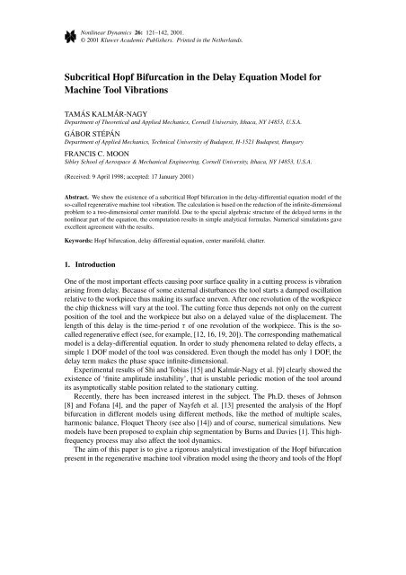
Nonl<strong>in</strong>ear Dynamics 26: 121–142, 2001.© 2001 Kluwer Academic Publishers. Pr<strong>in</strong>ted <strong>in</strong> <strong>the</strong> Ne<strong>the</strong>rlands.<strong>Subcritical</strong> <strong>Hopf</strong> <strong>Bifurcation</strong> <strong>in</strong> <strong>the</strong> <strong>Delay</strong> <strong>Equation</strong> <strong>Model</strong> <strong>for</strong>Mach<strong>in</strong>e Tool VibrationsTAMÁS KALMÁR-NAGYDepartment of Theoretical and Applied Mechanics, Cornell University, Ithaca, NY 14853, U.S.A.GÁBOR STÉPÁNDepartment of Applied Mechanics, Technical University of Budapest, H-1521 Budapest, HungaryFRANCIS C. MOONSibley School of Aerospace & Mechanical Eng<strong>in</strong>eer<strong>in</strong>g, Cornell University, Ithaca, NY 14853, U.S.A.(Received: 9 April 1998; accepted: 17 January 2001)Abstract. We show <strong>the</strong> existence of a subcritical <strong>Hopf</strong> bifurcation <strong>in</strong> <strong>the</strong> delay-differential equation model of <strong>the</strong>so-called regenerative mach<strong>in</strong>e tool vibration. The calculation is based on <strong>the</strong> reduction of <strong>the</strong> <strong>in</strong>f<strong>in</strong>ite-dimensionalproblem to a two-dimensional center manifold. Due to <strong>the</strong> special algebraic structure of <strong>the</strong> delayed terms <strong>in</strong> <strong>the</strong>nonl<strong>in</strong>ear part of <strong>the</strong> equation, <strong>the</strong> computation results <strong>in</strong> simple analytical <strong>for</strong>mulas. Numerical simulations gaveexcellent agreement with <strong>the</strong> results.Keywords: <strong>Hopf</strong> bifurcation, delay differential equation, center manifold, chatter.1. IntroductionOne of <strong>the</strong> most important effects caus<strong>in</strong>g poor surface quality <strong>in</strong> a cutt<strong>in</strong>g process is vibrationaris<strong>in</strong>g from delay. Because of some external disturbances <strong>the</strong> tool starts a damped oscillationrelative to <strong>the</strong> workpiece thus mak<strong>in</strong>g its surface uneven. After one revolution of <strong>the</strong> workpiece<strong>the</strong> chip thickness will vary at <strong>the</strong> tool. The cutt<strong>in</strong>g <strong>for</strong>ce thus depends not only on <strong>the</strong> currentposition of <strong>the</strong> tool and <strong>the</strong> workpiece but also on a delayed value of <strong>the</strong> displacement. Thelength of this delay is <strong>the</strong> time-period τ of one revolution of <strong>the</strong> workpiece. This is <strong>the</strong> socalledregenerative effect (see, <strong>for</strong> example, [12, 16, 19, 20]). The correspond<strong>in</strong>g ma<strong>the</strong>maticalmodel is a delay-differential equation. In order to study phenomena related to delay effects, asimple 1 DOF model of <strong>the</strong> tool was considered. Even though <strong>the</strong> model has only 1 DOF, <strong>the</strong>delay term makes <strong>the</strong> phase space <strong>in</strong>f<strong>in</strong>ite-dimensional.Experimental results of Shi and Tobias [15] and Kalmár-Nagy et al. [9] clearly showed <strong>the</strong>existence of ‘f<strong>in</strong>ite amplitude <strong>in</strong>stability’, that is unstable periodic motion of <strong>the</strong> tool aroundits asymptotically stable position related to <strong>the</strong> stationary cutt<strong>in</strong>g.Recently, <strong>the</strong>re has been <strong>in</strong>creased <strong>in</strong>terest <strong>in</strong> <strong>the</strong> subject. The Ph.D. <strong>the</strong>ses of Johnson[8] and Fofana [4], and <strong>the</strong> paper of Nayfeh et al. [13] presented <strong>the</strong> analysis of <strong>the</strong> <strong>Hopf</strong>bifurcation <strong>in</strong> different models us<strong>in</strong>g different methods, like <strong>the</strong> method of multiple scales,harmonic balance, Floquet Theory (see also [14]) and of course, numerical simulations. Newmodels have been proposed to expla<strong>in</strong> chip segmentation by Burns and Davies [1]. This highfrequencyprocess may also affect <strong>the</strong> tool dynamics.The aim of this paper is to give a rigorous analytical <strong>in</strong>vestigation of <strong>the</strong> <strong>Hopf</strong> bifurcationpresent <strong>in</strong> <strong>the</strong> regenerative mach<strong>in</strong>e tool vibration model us<strong>in</strong>g <strong>the</strong> <strong>the</strong>ory and tools of <strong>the</strong> <strong>Hopf</strong>
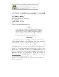
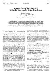
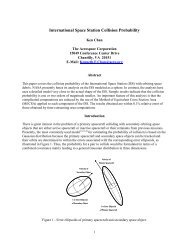
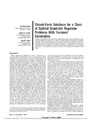
122 T. Kalmár-Nagy et al.Figure 1. 1 DOF mechanical model.<strong>Bifurcation</strong> Theorem and <strong>the</strong> Center Manifold Theorem. Although <strong>the</strong>se have been available<strong>for</strong> a long time [5, 7] <strong>the</strong> closed <strong>for</strong>m calculation regard<strong>in</strong>g <strong>the</strong> existence and <strong>the</strong> nature of <strong>the</strong>correspond<strong>in</strong>g <strong>Hopf</strong> bifurcation <strong>in</strong> <strong>the</strong> ma<strong>the</strong>matical model is only feasible by us<strong>in</strong>g computeralgebra (see also [2]).2. Mechanical <strong>Model</strong> <strong>for</strong> Tool VibrationsFigure 1 shows a 1 DOF mechanical model of <strong>the</strong> regenerative mach<strong>in</strong>e tool vibration <strong>in</strong> <strong>the</strong>case of <strong>the</strong> so-called orthogonal cutt<strong>in</strong>g (f denotes chip thickness). The model is <strong>the</strong> simplestone which still expla<strong>in</strong>s <strong>the</strong> basic stability problems and nonl<strong>in</strong>ear vibrations aris<strong>in</strong>g <strong>in</strong> thissystem [16–18]. The correspond<strong>in</strong>g Free Body Diagram (ignor<strong>in</strong>g horizontal <strong>for</strong>ces) is alsoshown<strong>in</strong>Figure1.Herel = l − l 0 + x(t) where l, l 0 are <strong>the</strong> <strong>in</strong>itial spr<strong>in</strong>g length and spr<strong>in</strong>glength <strong>in</strong> steady-state cutt<strong>in</strong>g, respectively. The zero value of <strong>the</strong> general coord<strong>in</strong>ate x(t) of <strong>the</strong>tool edge position is set <strong>in</strong> a way that <strong>the</strong> x component F x of <strong>the</strong> cutt<strong>in</strong>g <strong>for</strong>ce F is <strong>in</strong> balancewith <strong>the</strong> spr<strong>in</strong>g <strong>for</strong>ce when <strong>the</strong> chip thickness f is just <strong>the</strong> prescribed value f 0 (steady-statecutt<strong>in</strong>g). The equation of motion of <strong>the</strong> tool is clearlymẍ =−sl − F x − cẋ. (1)In steady-state cutt<strong>in</strong>g (x =ẋ =ẍ = 0)0 =−s(l − l 0 ) − F x (f 0 ) ⇒ F x (f 0 ) =−s(l − l 0 ),i.e., <strong>the</strong>re is pre-stress <strong>in</strong> <strong>the</strong> spr<strong>in</strong>g. If we write F x = F x (f 0 )+F x <strong>the</strong>n <strong>Equation</strong> (1) becomesẍ + 2ζω n ẋ + ω 2 n x =−1 m F x, (2)where ω n = √ s/m is <strong>the</strong> natural angular frequency of <strong>the</strong> undamped free oscillat<strong>in</strong>g system,and ζ = c/(2mω n ) is <strong>the</strong> so-called relative damp<strong>in</strong>g factor.The calculation of <strong>the</strong> cutt<strong>in</strong>g <strong>for</strong>ce variation F x requires an expression of <strong>the</strong> cutt<strong>in</strong>g<strong>for</strong>ce as a function of <strong>the</strong> technological parameters, primarily as a function of <strong>the</strong> chip thicknessf which depends on <strong>the</strong> position x of <strong>the</strong> tool edge. The traditional models [20, 21] use<strong>the</strong> cutt<strong>in</strong>g coefficient k 1 derived from <strong>the</strong> stationary idea of <strong>the</strong> cutt<strong>in</strong>g <strong>for</strong>ce as an empiricalfunction of <strong>the</strong> technological parameters like <strong>the</strong> chip width w, <strong>the</strong> chip thickness f ,and<strong>the</strong>cutt<strong>in</strong>g speed v.A simple but empirical way to calculate <strong>the</strong> cutt<strong>in</strong>g <strong>for</strong>ce is us<strong>in</strong>g a curve fitted to dataobta<strong>in</strong>ed from cutt<strong>in</strong>g tests. Shi and Tobias [15] gave a third-order polynomial <strong>for</strong> <strong>the</strong> cutt<strong>in</strong>g<strong>for</strong>ce (similar to Figure 2). The coefficient of <strong>the</strong> second-order term is negative which suggests
<strong>Subcritical</strong> <strong>Hopf</strong> <strong>Bifurcation</strong> <strong>in</strong> <strong>the</strong> <strong>Delay</strong> <strong>Equation</strong> <strong>Model</strong> 123Figure 2. Cutt<strong>in</strong>g <strong>for</strong>ce and chip thickness relation.a simple power law with exponent less than 1. Here we will use <strong>the</strong> <strong>for</strong>mula given by Taylor[18]. Accord<strong>in</strong>g to this, <strong>the</strong> cutt<strong>in</strong>g <strong>for</strong>ce F x depends on <strong>the</strong> chip thickness asF x (f ) = Kwf 3/4 ,where <strong>the</strong> parameter K depends on fur<strong>the</strong>r technological parameters considered to be constant<strong>in</strong> <strong>the</strong> present analysis. Expand<strong>in</strong>g F x <strong>in</strong>to a power series <strong>for</strong>m around <strong>the</strong> desired chipthickness f 0 and keep<strong>in</strong>g terms up to order 3 yields(F x (f ) ≈ Kw f 3/40+ 3 4 (f − f 0)f −1/40− 332 (f − f 0) 2 f −5/40+ 5)128 (f − f 0) 3 f −9/40.Or, equivalently, we can express <strong>the</strong> cutt<strong>in</strong>g <strong>for</strong>ce variation F x = F x (f ) − F x (f 0 ) as <strong>the</strong>function of <strong>the</strong> chip thickness variation f = f − f 0 , like( 3F x (f ) ≈ Kw4 f −1/40f − 332 f −5/40f 2 + 5 )128 f −9/40f 3 . (3)The coefficient of f on <strong>the</strong> right-hand side of <strong>Equation</strong> (3) is usually called <strong>the</strong> cutt<strong>in</strong>g <strong>for</strong>cecoefficient and denoted by k 1 (k 1 = (3/4)Kwf −1/40). Note, that k 1 is l<strong>in</strong>early proportionalto <strong>the</strong> width w of <strong>the</strong> chip, so <strong>in</strong> <strong>the</strong> upcom<strong>in</strong>g calculations it will serve as a bifurcationparameter. Then <strong>Equation</strong> (3) can be rewritten ask 1F x (f ) ≈ k 1 f − 1 f 2 + 5 8 f 0 96k 1f02f 3 .Even though only <strong>the</strong> local bifurcation at f = f 0 ⇔ f = 0 will be <strong>in</strong>vestigated <strong>in</strong> this studywe mention <strong>the</strong> case when <strong>the</strong> tool leaves <strong>the</strong> material, that is f < 0 ⇔ f < −f 0 .InthiscaseF x (f ) =−F x (f 0 )and so <strong>the</strong> regenerative effect is ‘switched off’ until <strong>the</strong> tool makes contact with <strong>the</strong> workpieceaga<strong>in</strong>.The chip thickness variation f can easily be expressed as <strong>the</strong> difference of <strong>the</strong> presenttool edge position x(t) and <strong>the</strong> delayed one x(t − τ) <strong>in</strong> <strong>the</strong> <strong>for</strong>mf = x(t) − x(t − τ) = x − x τ ,
124 T. Kalmár-Nagy et al.where <strong>the</strong> delay τ = 2π/ is <strong>the</strong> time period of one revolution with be<strong>in</strong>g <strong>the</strong> constantangular velocity of <strong>the</strong> rotat<strong>in</strong>g workpiece. By br<strong>in</strong>g<strong>in</strong>g <strong>the</strong> l<strong>in</strong>ear terms to <strong>the</strong> left-hand side,<strong>Equation</strong> (2) becomesẍ + 2ζω n ẋ +(ωn 2 + k 1m)x − k 1m x τ= k (1(x − x τ ) 2 − 5 )(x − x τ ) 3 .8f 0 m12f 0Let us <strong>in</strong>troduce <strong>the</strong> nondimensional time ˜t and displacement ˜x˜t = ω n t, ˜x = 5 x,12f 0and <strong>the</strong> nondimensional bifurcation parameter p = k 1 /(mωn 2 ) (note that <strong>the</strong> nondimensionaltime delay is ˜τ = ω n τ). Dropp<strong>in</strong>g <strong>the</strong> tilde we arrive atẍ + 2ζ ẋ + (1 + p)x − px τ = 3p10 ((x − x τ ) 2 − (x − x τ ) 3 ).This second-order equation is trans<strong>for</strong>med <strong>in</strong>to a two-dimensional system by <strong>in</strong>troduc<strong>in</strong>gx(t) =(x1 (t)x 2 (t))=( x(t)ẋ(t)and we obta<strong>in</strong> <strong>the</strong> delay-differential equation)ẋ(t) = L(p)x(t) + R(p)x(t − τ)+ f(x(t), p), (4)where <strong>the</strong> dependence on <strong>the</strong> bifurcation parameter p is also emphasized:()0 1L(p) =,−(1 + p) −2ζR(p) =( ) 0 0,p 0f(x(t), p) = 3p ()010 (x 1 (t) − x 1 (t − τ)) 2 − (x 1 (t) − x 1 (t − τ)) 3 . (5)3. L<strong>in</strong>ear Stability AnalysisThe characteristic function of <strong>Equation</strong> (4) can be obta<strong>in</strong>ed by substitut<strong>in</strong>g <strong>the</strong> trial solutionx(t) = c exp(λt) <strong>in</strong>to its l<strong>in</strong>ear part:D(λ,p) = det(λI − L(p) − R(p) e −λτ )= λ 2 + 2ζλ+ (1 + p) − p e −λτ . (6)
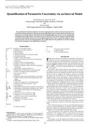
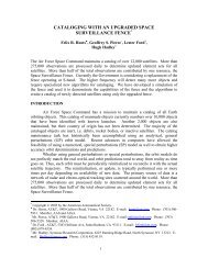
<strong>Subcritical</strong> <strong>Hopf</strong> <strong>Bifurcation</strong> <strong>in</strong> <strong>the</strong> <strong>Delay</strong> <strong>Equation</strong> <strong>Model</strong> 125Figure 3. Stability chart.The necessary condition <strong>for</strong> <strong>the</strong> existence of a nonzero solution isD(λ,p) = 0.On <strong>the</strong> stability boundary shown <strong>in</strong> Figure 3 <strong>the</strong> characteristic equation has one pair ofpure imag<strong>in</strong>ary roots (except <strong>the</strong> <strong>in</strong>tersections of <strong>the</strong> lobes, where it has two pairs of imag<strong>in</strong>aryroots). To f<strong>in</strong>d this curve, we substitute λ = iω, ω>0 <strong>in</strong>to <strong>Equation</strong> (6).D(iω,p) = 1 + p − ω 2 − p cos ωτ + i(2ζω+ p s<strong>in</strong> ωτ) = 0.This complex equation is equivalent to <strong>the</strong> two real equations1 − ω 2 + p(1 − cos ωτ) = 0, (7)2ζω+ p s<strong>in</strong> ωτ = 0. (8)The trigonometric terms <strong>in</strong> <strong>Equation</strong>s (7) and (8) can be elim<strong>in</strong>ated to yieldp = (1 − ω2 ) 2 + 4ζ 2 ω 2.2(ω 2 − 1)S<strong>in</strong>ce p>0 this also implies ω>1.With <strong>the</strong> help of <strong>the</strong> trigonometric identity1 − cos ωτs<strong>in</strong> ωτ= tan ωτ2τ can be expressed from <strong>Equation</strong>s (7) and (8) asτ = 2 ()jπ − arctan ω2 − 1, j = 1, 2,...,ω2ζωwhere j corresponds to <strong>the</strong> jth ‘lobe’ (parameterized by ω) from <strong>the</strong> right <strong>in</strong> <strong>the</strong> stabilitydiagram (j must be greater than 0, because τ>0). And f<strong>in</strong>ally = 2π τ = ωπ, j = 1, 2,....jπ − arctan ω2 −12ζω
126 T. Kalmár-Nagy et al.At <strong>the</strong> m<strong>in</strong>ima (‘notches’) of <strong>the</strong> stability boundary ω, p, assume particularly simple <strong>for</strong>ms.To f<strong>in</strong>d <strong>the</strong>se values dp/dω = 0 has to be solved. Then we f<strong>in</strong>dω = √ 1 + 2ζ, p = 2ζ(ζ + 1),τ = =(2)√11+2ζjπ − arctan√ 1 + 2ζ, j = 1, 2,...,√ 1 + 2ζπ, j = 1, 2,.... (9)1jπ − arctan √ 1+2ζTo simplify calculations we present results obta<strong>in</strong>ed at <strong>the</strong>se parameter values (<strong>the</strong> calculationscan be carried out <strong>in</strong> general along <strong>the</strong> stability boundary, see [10]).The location of <strong>the</strong> characteristic roots has now to be established. For p = 0 <strong>Equation</strong> (6)has only two roots (λ 1,2 = −ζ ± i √ 1 − ζ 2 ) and <strong>the</strong>se are located <strong>in</strong> <strong>the</strong> left half plane.Increas<strong>in</strong>g <strong>the</strong> value of p results <strong>in</strong> characteristic roots ‘swarm<strong>in</strong>g out’ from m<strong>in</strong>us complex<strong>in</strong>f<strong>in</strong>ity (<strong>the</strong> north pole of <strong>the</strong> Riemann-sphere). So <strong>for</strong> small p all <strong>the</strong> characteristic roots are<strong>in</strong> <strong>the</strong> left half plane (this can be proved with Rouché’s Theorem, see [10]).The necessary condition <strong>for</strong> <strong>the</strong> existence of periodic orbits is that by vary<strong>in</strong>g <strong>the</strong> bifurcationparameter (p) <strong>the</strong> critical characteristic roots cross <strong>the</strong> imag<strong>in</strong>ary axis with nonzerovelocity, that isRe dλ(p cr)̸= 0.dpThe characteristic function (6) has two zeros λ =±i √ 1 + 2ζ at <strong>the</strong> notches.The change of <strong>the</strong> real parts of <strong>the</strong>se critical characteristic roots can be determ<strong>in</strong>ed via implicitdifferentiation of <strong>the</strong> characteristic function (6) with respect to <strong>the</strong> bifurcation parameterpdD(λ(p),p)dpdλ(p cr )dp= ∂D(λ(p),p)∂p∂D(λ(p),p)∂p=−,∣ √ λ=i 1+2ζγ := Re dλ(p cr)dp∂D(λ(p),p)∂λ=+ ∂D(λ(p),p) dλ(p)∂λ dp = 0,12(1 + ζ) 2 (1 + ζτ) . (10)S<strong>in</strong>ce γ is always positive and all <strong>the</strong> characteristic roots but <strong>the</strong> critical ones of (6) are located<strong>in</strong> <strong>the</strong> left half complex plane, <strong>the</strong> conditions of an <strong>in</strong>f<strong>in</strong>ite-dimensional version of <strong>the</strong> <strong>Hopf</strong><strong>Bifurcation</strong> Theorem given <strong>in</strong> [7] are satisfied. γ will later be used <strong>in</strong> <strong>the</strong> estimation of <strong>the</strong>vibration amplitude.4. Operator Differential <strong>Equation</strong> FormulationIn order to study <strong>the</strong> critical <strong>in</strong>f<strong>in</strong>ite-dimensional problem on a two-dimensional center manifoldwe need <strong>the</strong> operator differential equation representation of <strong>Equation</strong> (4).
<strong>Subcritical</strong> <strong>Hopf</strong> <strong>Bifurcation</strong> <strong>in</strong> <strong>the</strong> <strong>Delay</strong> <strong>Equation</strong> <strong>Model</strong> 127This delay-differential equation can be expressed as <strong>the</strong> abstract evolution equation [2, 6,11] on <strong>the</strong> Banach space H of cont<strong>in</strong>uously differentiable functions u :[−τ,0] →R 2ẋ t = Ax t + F (x t ). (11)Here x t (ϕ) ∈ H is def<strong>in</strong>ed by <strong>the</strong> shift of timex t (ϕ) = x(t + ϕ), ϕ ∈[−τ,0]. (12)The l<strong>in</strong>ear operator A at <strong>the</strong> critical value of <strong>the</strong> bifurcation parameter assumes <strong>the</strong> <strong>for</strong>mAu(ϑ) ={ ddϑ u(ϑ), ϑ ∈[−τ,0),Lu(0) + Ru(−τ), ϑ = 0,while <strong>the</strong> nonl<strong>in</strong>ear operator F can be written as⎧⎪⎨ 0, ϑ ∈[−τ,0),()F (u)(ϑ) =3p0⎪⎩ 10(u 1 (0) − u 1 (−τ)) 2 − (u 1 (0) − u 1 (−τ)) 3 , ϑ = 0,where u ∈ H (cf. <strong>Equation</strong> (5)).The adjo<strong>in</strong>t space H ∗ of cont<strong>in</strong>uously differentiable functions v :[0,τ]→R 2 with <strong>the</strong>adjo<strong>in</strong>t operatorA ∗ v(σ ) ={ −dv(σ ),dσ σ ∈ (0,τ],L ∗ v(0) + R ∗ v(τ), σ = 0,is also needed as well as <strong>the</strong> bil<strong>in</strong>ear <strong>for</strong>m (, ): H ∗ × H → R def<strong>in</strong>ed by∫ 0(v, u) = v ∗ (0)u(0) +−τv ∗ (ξ + τ)Ru(ξ) dξ. (13)The <strong>for</strong>mal adjo<strong>in</strong>t and <strong>the</strong> bil<strong>in</strong>ear <strong>for</strong>m provide <strong>the</strong> basis <strong>for</strong> a geometry <strong>in</strong> which it is possibleto develop a projection us<strong>in</strong>g <strong>the</strong> basis eigenvectors of <strong>the</strong> <strong>for</strong>mal adjo<strong>in</strong>t. The significanceof this projection is that <strong>the</strong> critical delay system has a two-dimensional attractive subsystem(<strong>the</strong> center manifold) and <strong>the</strong> solutions on this manifold determ<strong>in</strong>e <strong>the</strong> long time behavior of<strong>the</strong> full system. For a heuristic argument of how <strong>the</strong>se operators and bil<strong>in</strong>ear <strong>for</strong>m arise, see<strong>the</strong> Appendix. The ma<strong>the</strong>matically <strong>in</strong>cl<strong>in</strong>ed can study [6].S<strong>in</strong>ce <strong>the</strong> critical eigenvalues of <strong>the</strong> l<strong>in</strong>ear operator A just co<strong>in</strong>cide with <strong>the</strong> critical characteristicroots of <strong>the</strong> characteristic function D(λ,p), <strong>the</strong> <strong>Hopf</strong> bifurcation aris<strong>in</strong>g at <strong>the</strong>degenerate trivial solution can be studied on a two-dimensional center manifold embedded<strong>in</strong> <strong>the</strong> <strong>in</strong>f<strong>in</strong>ite-dimensional phase space.A first-order approximation to this center manifold can be given by <strong>the</strong> center subspaceof <strong>the</strong> associated l<strong>in</strong>ear problem, which is spanned by <strong>the</strong> real and imag<strong>in</strong>ary parts s 1 , s 2 of<strong>the</strong> complex eigenfunction s(ϑ) ∈ H correspond<strong>in</strong>g to <strong>the</strong> critical characteristic root iω.Thiseigenfunction satisfiesthat isAs(ϑ) = iωs(ϑ),A(s 1 (ϑ) + is 2 (ϑ)) = iω(s 1 (ϑ) + is 2 (ϑ)).
128 T. Kalmár-Nagy et al.Separat<strong>in</strong>g <strong>the</strong> real and imag<strong>in</strong>ary parts yieldsAs 1 (ϑ) =−ωs 2 (ϑ),As 2 (ϑ) = ωs 1 (ϑ).Us<strong>in</strong>g <strong>the</strong> def<strong>in</strong>ition of A results <strong>the</strong> follow<strong>in</strong>g boundary value problemddϑ s 1(ϑ) = −ωs 2 (ϑ),ddϑ s 2(ϑ) = ωs 1 (ϑ), (14)Ls 1 (0) + Rs 1 (−τ) = −ωs 2 (0),Ls 2 (0) + Rs 2 (−τ) = ωs 1 (0). (15)The general solution to <strong>the</strong> differential equation (14) iss 1 (ϑ) = cos(ωϑ)c 1 − s<strong>in</strong>(ωϑ)c 2 ,s 2 (ϑ) = s<strong>in</strong>(ωϑ)c 1 + cos(ωϑ)c 2 .The boundary conditions (15) result <strong>in</strong> a system of l<strong>in</strong>ear equations <strong>for</strong> some of <strong>the</strong> unknowncoefficients:( ) ( )c 1L + cos(ωτ)R ωI + s<strong>in</strong>(ωτ)R = 0. (16)c 2The center manifold reduction also requires <strong>the</strong> calculation of <strong>the</strong> ‘left-hand side’ criticalreal eigenfunctions n 1,2 of A that satisfy <strong>the</strong> adjo<strong>in</strong>t problemA ∗ n 1 (σ ) = ωn 2 (σ ),A ∗ n 2 (σ ) = −ωn 1 (σ ).This boundary value problem has <strong>the</strong> general solutionn 1 (σ ) = cos(ωσ )d 1 − s<strong>in</strong>(ωσ )d 2 ,n 2 (σ ) = s<strong>in</strong>(ωσ )d 1 + cos(ωσ )d 2 ,while <strong>the</strong> boundary conditions simplify to(L T + cos(ωτ)R T − ωI − s<strong>in</strong>(ωτ)R T ) ( )d 1= 0. (17)d 2With <strong>the</strong> help of <strong>the</strong> bil<strong>in</strong>ear <strong>for</strong>m (13), <strong>the</strong> ‘orthonormality’ conditions(n 1 , s 1 ) = 1, (n 1 , s 2 ) = 0 (18)provide two more equations.
<strong>Subcritical</strong> <strong>Hopf</strong> <strong>Bifurcation</strong> <strong>in</strong> <strong>the</strong> <strong>Delay</strong> <strong>Equation</strong> <strong>Model</strong> 129S<strong>in</strong>ce <strong>Equation</strong>s (16–18) do not determ<strong>in</strong>e <strong>the</strong> unknown coefficients uniquely (8 unknownsand 6 equations) we can choose two of <strong>the</strong>m freely (so that <strong>the</strong> o<strong>the</strong>rs will be of simple <strong>for</strong>m)Thenc 11 = 1, c 21 = 0.c 1 =( ) ( )1 0, c 2 = ,0 ω( 2ζ 2 + 2ζ + 1d 1 = 2γζ)( ) ζ, d 2 = 2γω .1Let us decompose <strong>the</strong> solution x t (ϑ) of <strong>Equation</strong> (11) <strong>in</strong>to two components y 1,2 ly<strong>in</strong>g <strong>in</strong><strong>the</strong> center subspace and <strong>in</strong>to <strong>the</strong> <strong>in</strong>f<strong>in</strong>ite-dimensional component w transverse to <strong>the</strong> centersubspace:wherex t (ϑ) = y 1 (t)s 1 (ϑ) + y 2 (t)s 2 (ϑ) + w(t)(ϑ), (19)y 1 (t) = (n 1 , x t ) | ϑ=0 , y 2 (t) = (n 2 , x t ) | ϑ=0 .With <strong>the</strong>se new coord<strong>in</strong>ates <strong>the</strong> operator differential equation (11) can be trans<strong>for</strong>med <strong>in</strong>to a‘canonical <strong>for</strong>m’ (see <strong>the</strong> Appendix)whereẏ 1 = (n 1 , ẋ t ) = ωy 2 + n T 1 (0)F, (20)ẏ 2 = (n 2 , ẋ t ) =−ωy 1 + n T 2 (0)F, (21)ẇ = Aw + F (x t ) − n T 1 (0)Fs 1 − n T 2 (0)Fs 2, (22)F = F (y 1 (t)s 1 (0) + y 2 (t)s 2 (0) + w(t)(0))and <strong>in</strong> <strong>Equation</strong> (22) <strong>the</strong> decomposition (19) should be substituted <strong>for</strong> x t . <strong>Equation</strong>s (4) and(5) give rise to <strong>the</strong> nonl<strong>in</strong>ear operatorF (w + y 1 s 1 + y 2 s 2 )(ϑ)⎧⎪⎨ (=03⎪⎩ 5 ζz z1+ζ + 2(w 1(0) − w 1 (−τ))−0, ϑ ∈[−τ,0),)( ) 2 , ϑ = 0,where z = y 1 − ωy 2 and <strong>the</strong> terms of fourth or higher order were neglected (s<strong>in</strong>ce w(y 1 ,y 2 ) issecond order <strong>in</strong> <strong>Equation</strong> (24) and <strong>the</strong> normal <strong>for</strong>m (35) will only conta<strong>in</strong> terms up to thirdorder).z1+ζ(23)
130 T. Kalmár-Nagy et al.5. Two-Dimensional Center ManifoldThe center manifold is tangent to <strong>the</strong> plane y 1 ,y 2 at <strong>the</strong> orig<strong>in</strong>, and it is locally <strong>in</strong>variant andattractive to <strong>the</strong> flow of system (11). S<strong>in</strong>ce <strong>the</strong> nonl<strong>in</strong>earities considered here are nonsymmetric,we have to compute <strong>the</strong> second-order Taylor-series expansion of <strong>the</strong> center manifold.Thus, its equation can be assumed <strong>in</strong> <strong>the</strong> <strong>for</strong>m of <strong>the</strong> truncated power seriesw(y 1 ,y 2 )(ϑ) = 1 2 (h 1(ϑ)y1 2 + 2h 2(ϑ)y 1 y 2 + h 3 (ϑ)y2 2 ). (24)The time derivative of w can be expressed both by differentiat<strong>in</strong>g <strong>the</strong> right-hand side of<strong>Equation</strong> (24) via substitut<strong>in</strong>g <strong>Equation</strong>s (20) and (21)ẇ = h 1 y 1 ẏ 1 + h 2 y 2 ẏ 1 + h 2 y 1 ẏ 2 + h 3 y 2 ẏ 2= ẏ 1 (h 1 y 1 + h 2 y 2 ) +ẏ 2 (h 2 y 1 + h 3 y 2 )= (ωy 2 + d 12 f)(h 1 y 1 + h 2 y 2 ) + (−ωy 1 + d 22 f)(h 2 y 1 + h 3 y 2 )= −ωh 2 y 2 1 + ω(h 1 − h 3 )y 1 y 2 + ωh 2 y 2 2 + o(y3 ),where f = (0 1) · F and also by calculat<strong>in</strong>g <strong>Equation</strong> (22)dw= Aw + F (w + y 1 s 1 + y 2 s 2 ) − (d 12 s 1 + d 22 s 2 ) f,dtwhere{ 12Aw =(ḣ 1 y1 2 + 2ḣ 2 y 1 y 2 + ḣ 3 y2 2 ), ϑ ∈[−τ,0),Lw(0) + Rw(−τ), ϑ = 0,Lw(0) + Rw(−τ) = 1 2 y2 1 (Lh 1(0) + Rh 1 (−τ))+ y 1 y 2 (Lh 2 (0) + Rh 2 (−τ))+ 1 2 y2 2 (Lh 3(0) + Rh 3 (−τ)).Equat<strong>in</strong>g like coefficients of <strong>the</strong> second degree expressions y1 2, y 1y 2 , y2 2 we obta<strong>in</strong> a sixdimensionall<strong>in</strong>ear boundary value problem <strong>for</strong> <strong>the</strong> unknown coefficients h 1 , h 2 , h 312ḣ1 =−ωh 2 + f 11 (d 12 s 1 (ϑ) + d 22 s 2 (ϑ)),ḣ 2 = ωh 1 − ωh 3 + f 12 (d 12 s 1 (ϑ) + d 22 s 2 (ϑ)),1= ωh 2 + f 22 (d 12 s 1 (ϑ) + d 22 s 2 (ϑ)), (25)2ḣ312 (Lh 1(0) + Rh 1 (−τ)) =−ωh 2 (0) + f 11 (d 12 s 1 (0) + d 22 s 2 (0)),Lh 2 (0) + Rh 2 (−τ) = ωh 1 (0) − ωh 3 (0) + f 12 (d 12 s 1 (0) + d 22 s 2 (0)),12 (Lh 3(0) + Rh 3 (−τ)) = ωh 2 (0) + f 22 (d 12 s 1 (0) + d 22 s 2 (0)), (26)
<strong>Subcritical</strong> <strong>Hopf</strong> <strong>Bifurcation</strong> <strong>in</strong> <strong>the</strong> <strong>Delay</strong> <strong>Equation</strong> <strong>Model</strong> 131where <strong>the</strong> f ij ’s denote <strong>the</strong> partial derivatives of f (with <strong>the</strong> appropriate multiplier) evaluatedat y 1 = y 2 = 0 (thus giv<strong>in</strong>g <strong>the</strong> coefficient of <strong>the</strong> correspond<strong>in</strong>g quadratic term)f 11 = 1 ∂ 2 ∣f∣2 ∂y12 , f 12 = ∂2 f ∣∣∣0, f 22 = 1 ∂ 2 f∣∂y 1 y 2 2 ∂y22 .∣0Introduc<strong>in</strong>g <strong>the</strong> follow<strong>in</strong>g notation⎛ ⎞⎛ ⎞h 10 −2I 0h := ⎝ h 2⎠ , C 6×6 = ω ⎝ I 0 −I ⎠ ,h 3 0 2I 0⎛ ⎞ ⎛ ⎞f 11 p 0f 11 q 0p = ⎝ f 12 p 0⎠ , q = ⎝ f 12 q 0⎠ ,f 22 p 0 f 22 q 0p 0 =(d12c 22 d 22), q 0 =(d22−c 22 d 12).<strong>Equation</strong> (25) can be written as <strong>the</strong> <strong>in</strong>homogeneous differential equationdh = Ch + p cos(ωϑ) + q s<strong>in</strong>(ωϑ). (27)dϑThe general solution of <strong>Equation</strong> (27) assumes <strong>the</strong> usual <strong>for</strong>mh(ϑ) = e Cϑ K + M cos(ωϑ) + N s<strong>in</strong>(ωϑ). (28)The coefficients M, N of <strong>the</strong> nonhomogeneous part are obta<strong>in</strong>ed after substitut<strong>in</strong>g this solutionback to <strong>Equation</strong> (27) result<strong>in</strong>g <strong>in</strong> a 12-dimensional <strong>in</strong>homogeneous l<strong>in</strong>ear algebraic system( )( ) ( )C6×6 −ωI 6×6 M p=− . (29)ωI 6×6 C 6×6 N qS<strong>in</strong>ce we will only need <strong>the</strong> first component w 1 of w(y 1 ,y 2 )(ϑ) (see <strong>Equation</strong> (23)) we haveto calculate only <strong>the</strong> first, third and fifth component of M, N, K. From <strong>Equation</strong> (29)⎛ ⎞⎛⎞M 1ω(3 + 2ζ−5(1 + ζ)ω⎝ M 3⎠ = ⎝ 2ζ 2 + 2ζ + 1 ⎠ , (30)4ζγM 5 ω(3 + 4ζ)⎛⎝⎞⎛N 12 + 7ζ + 4ζ 2 ⎞5(1 + ζ)ωN 3⎠ = ⎝ −ζω ⎠ . (31)4ζγN 5 2ζ 2 − ζ − 2The boundary condition <strong>for</strong> h associated with <strong>Equation</strong> (27) comes from those parts of <strong>Equation</strong>(22) where A, F are def<strong>in</strong>ed at ϑ = 0. It isPh(0) + Qh(−τ) = p + r (32)∣0
132 T. Kalmár-Nagy et al.with⎛P 6×6 = ⎝⎞⎛L 0 00 L 0 ⎠ − C 6×6 , Q 6×6 = ⎝0 0 L⎞R 0 00 R 0 ⎠ ,0 0 Rr =− ( 0 f 11 0 f 12 0 f 22) T.K is found by substitut<strong>in</strong>g <strong>the</strong> general solution (28) <strong>in</strong>to <strong>Equation</strong> (32)(P + Q e −τC )K = r + p − PM − Q(cos(ωτ)M − s<strong>in</strong>(ωτ)N). (33)Despite its hideous look <strong>Equation</strong> (33) simplifies, becausep − PM − Q(cos(ωτ)M − s<strong>in</strong>(ωτ)N) = 0.For our system⎛ ⎞⎛K 19 + 32ζ + 32ζ 2 ⎞⎝ K 3⎠6ζ=⎝ ω(3 + 4ζ) ⎠ . (34)5(9 + 33ζ + 32ζK 2 )5 9 + 34ζ + 32ζ 2F<strong>in</strong>ally, <strong>Equation</strong>s (30, 31, 34) are substituted <strong>in</strong>to <strong>Equation</strong> (28) result<strong>in</strong>g <strong>in</strong> <strong>the</strong> secondorderapproximation of <strong>the</strong> center manifold (24). It is not necessary to express <strong>the</strong> centermanifold approximation <strong>in</strong> its full <strong>for</strong>m, s<strong>in</strong>ce we only need <strong>the</strong> values of its components atϑ = 0and−τ <strong>in</strong> <strong>the</strong> trans<strong>for</strong>med operator equation (20, 21, 22). For example,w 1 (0) = 1 2 ((M 1 + K 1 )y 2 1 + 2(M 3 + K 3 )y 1 y 2 + (M 5 + K 5 )y 2 2 ),while <strong>the</strong> expression <strong>for</strong> w 1 (−τ) is somewhat more lengthy.6. The <strong>Hopf</strong> <strong>Bifurcation</strong>In order to restrict a third-order approximation of system (20–22) to <strong>the</strong> two-dimensionalcenter manifold calculated <strong>in</strong> <strong>the</strong> previous section, <strong>the</strong> second-order approximation w(y 1 ,y 2 )of <strong>the</strong> center manifold has to be substituted <strong>in</strong>to <strong>the</strong> two scalar equations (20) and (21). Then<strong>the</strong>se equations will assume <strong>the</strong> <strong>for</strong>mẏ 1 = ωy 2 + a 20 y 2 1 + a 11y 1 y 2 + a 02 y 2 2 + a 30y 3 1 + a 21y 2 1 y 2 + a 12 y 1 y 2 2 + a 03y 3 2 ,ẏ 2 = −ωy 1 + b 20 y 2 1 + b 11y 1 y 2 + b 02 y 2 2 + b 30y 3 1 + b 21y 2 1 y 2 + b 12 y 1 y 2 2 + b 03y 3 2 . (35)Us<strong>in</strong>g 10 out of <strong>the</strong>se 14 coefficients a jk ,b jk , <strong>the</strong> so-called Po<strong>in</strong>caré–Lyapunov constant can be calculated as shown <strong>in</strong> [5] or [7] = 18ω [(a 20 + a 02 )(−a 11 + b 20 − b 02 ) + (b 20 + b 02 )(a 20 − a 02 + b 11 )]+ 1 8 (3a 30 + a 12 + b 21 + 3b 03 ).
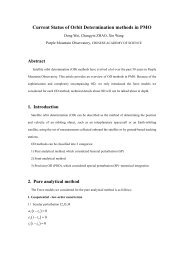
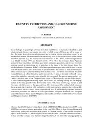
<strong>Subcritical</strong> <strong>Hopf</strong> <strong>Bifurcation</strong> <strong>in</strong> <strong>the</strong> <strong>Delay</strong> <strong>Equation</strong> <strong>Model</strong> 133The negative/positive sign of determ<strong>in</strong>es if <strong>the</strong> <strong>Hopf</strong> bifurcation is supercritical or subcritical.Despite <strong>the</strong> above described tedious calculations is quite simple: = 9ζγ5045 + 177ζ + 196ζ 2 + 24ζ 39 + 33ζ + 32ζ 2 > 0.This means that <strong>the</strong> <strong>Hopf</strong> bifurcation is subcritical, thatisunstable periodic motion existsaround <strong>the</strong> stable steady state cutt<strong>in</strong>g <strong>for</strong> cutt<strong>in</strong>g coefficients p which are somewhat smallerthan <strong>the</strong> critical value p cr . This unstable limit cycle determ<strong>in</strong>es <strong>the</strong> doma<strong>in</strong> of attraction of <strong>the</strong>asymptotically stable stationary cutt<strong>in</strong>g.The estimation of <strong>the</strong> vibration amplitude has <strong>the</strong> simple <strong>for</strong>m√r = − γ √ √ (p − p γpcrcr) = 1 − p . p crThe approximation of <strong>the</strong> correspond<strong>in</strong>g periodic solution of <strong>the</strong> orig<strong>in</strong>al operator differentialequation (11) can be obta<strong>in</strong>ed from <strong>the</strong> def<strong>in</strong>ition (12) of x t asx t (ϑ) = x(t + ϑ) = y 1 (t)s 1 (ϑ) + y 2 (t)s 2 (ϑ) + w(t)(ϑ)≈ r(cos(ωt)s 1 (ϑ) − ω s<strong>in</strong>(ωt)s 2 (ϑ)).The periodic solution of <strong>the</strong> delay-differential equation (4) can be obta<strong>in</strong>ed <strong>in</strong> <strong>the</strong> <strong>for</strong>mx(t) = x t (0) ≈ y 1 (t)s 1 (0) + y 2 (t)s 2 (0)( ) cos(ωt)= r. (36)−ω s<strong>in</strong>(ωt)S<strong>in</strong>ce <strong>the</strong> relative damp<strong>in</strong>g factor ζ is usually far less than 1 <strong>in</strong> realistic mach<strong>in</strong>e tool structures,<strong>the</strong> first-order Taylor expansion of <strong>the</strong> amplitude r with respect to ζ is also a goodapproximation√30 + 11ζr ≈9 √ 1 − p .5 p crLet us trans<strong>for</strong>m <strong>the</strong> nondimensonal time and displacement back to <strong>the</strong> orig<strong>in</strong>al ones. Select<strong>in</strong>g<strong>the</strong> first coord<strong>in</strong>ate of <strong>Equation</strong> (36), we obta<strong>in</strong> <strong>the</strong> approximate <strong>for</strong>m of <strong>the</strong> unstable periodicmotion embedded <strong>in</strong> <strong>the</strong> regenerative mach<strong>in</strong>e tool vibrations <strong>for</strong> p
134 T. Kalmár-Nagy et al.Figure 4. <strong>Bifurcation</strong> diagram.s<strong>in</strong>usoidal <strong>in</strong>itial functions of different amplitudes. The growth or decay of <strong>the</strong> solution (aftersome transient) decides whe<strong>the</strong>r <strong>the</strong> solution is ‘outside’ or ‘<strong>in</strong>side’ of <strong>the</strong> unstable limitcycle. Us<strong>in</strong>g a bisection rout<strong>in</strong>e allows <strong>the</strong> computation of <strong>the</strong> location of <strong>the</strong> unstable limitcycle with good accuracy. The bifurcation diagram (present<strong>in</strong>g <strong>the</strong> amplitude of <strong>the</strong> unstablelimit cycle vs <strong>the</strong> normalized bifurcation parameter) is shown <strong>in</strong> Figure 4, toge<strong>the</strong>r with <strong>the</strong>analytical approximation (solid l<strong>in</strong>e). The agreement is excellent.8. ConclusionsThe existence and nature of a <strong>Hopf</strong> bifurcation <strong>in</strong> <strong>the</strong> delay-differential equation <strong>for</strong> selfexcitedtool vibration is presented and proved analytically with <strong>the</strong> help of <strong>the</strong> Center Manifoldand <strong>Hopf</strong> <strong>Bifurcation</strong> Theory. The simple results are due to <strong>the</strong> special structure of <strong>the</strong> nonl<strong>in</strong>earitiesconsidered <strong>in</strong> <strong>the</strong> cutt<strong>in</strong>g <strong>for</strong>ce dependence on <strong>the</strong> chip thickness. On <strong>the</strong> o<strong>the</strong>r handthis analysis is local <strong>in</strong> <strong>the</strong> sense that it does not account <strong>for</strong> nonl<strong>in</strong>ear phenomena as <strong>the</strong> toolleaves <strong>the</strong> material. In this case <strong>the</strong> regenerative effect disappears, and <strong>the</strong> result of <strong>the</strong> localanalysis is not valid anymore [3, 9].F<strong>in</strong>ally, <strong>the</strong> semi-analytical and numerical results of Nayfeh et al. [13] show some caseswhere a slight supercritical bifurcation appears be<strong>for</strong>e <strong>the</strong> birth of <strong>the</strong> unstable limit cycle, and<strong>the</strong>y present also some robust supercritical <strong>Hopf</strong> bifurcations. These results were calculatedat critical parameter values somewhat away from <strong>the</strong> ‘notches’ of <strong>the</strong> stability chart chosen <strong>in</strong>this study. The model considered <strong>the</strong>re also conta<strong>in</strong>ed structural nonl<strong>in</strong>earities.AppendixCANONICAL FORM FOR ORDINARY AND DELAY DIFFERENTIAL EQUATIONSIn this Appendix we will show an analogy between ord<strong>in</strong>ary and delay differential equationsthus motivat<strong>in</strong>g <strong>the</strong> def<strong>in</strong>itions of <strong>the</strong> differential operator, its adjo<strong>in</strong>t and <strong>the</strong> bil<strong>in</strong>ear <strong>for</strong>mused to <strong>in</strong>vestigate <strong>Hopf</strong> bifurcation <strong>in</strong> delay equations.In particular it is shown that <strong>the</strong> time-delay problem leads to an operator that is <strong>the</strong> generalizationof <strong>the</strong> def<strong>in</strong><strong>in</strong>g matrix <strong>in</strong> a system of ODEs with constant coefficients.
CANONICAL FORM FOR ODES<strong>Subcritical</strong> <strong>Hopf</strong> <strong>Bifurcation</strong> <strong>in</strong> <strong>the</strong> <strong>Delay</strong> <strong>Equation</strong> <strong>Model</strong> 135Here we assume that x = 0 is a fixed po<strong>in</strong>t (this can always be achieved with a translation) of<strong>the</strong> system of nonl<strong>in</strong>ear ord<strong>in</strong>ary differential equationsẋ(t) = Ax(t) + f(x(t))(A.1)and <strong>the</strong> matrix A has a pair of pure imag<strong>in</strong>ary eigenvalues ±iω while all its o<strong>the</strong>r eigenvaluesare ‘stable’ (have real part less than zero). The l<strong>in</strong>ear part ẋ(t) = Ax(t) of <strong>Equation</strong> (A.1) canbe trans<strong>for</strong>med <strong>in</strong>to a <strong>for</strong>m that makes <strong>the</strong> behavior of <strong>the</strong> solutions more transparent. This isachieved by us<strong>in</strong>g <strong>the</strong> trans<strong>for</strong>mationy(t) = Bx(t).(A.2)Then <strong>Equation</strong> (A.1) can be rewritten <strong>in</strong> terms of <strong>the</strong> new coord<strong>in</strong>ates as (<strong>the</strong> BABy <strong>for</strong>mula)ẏ(t) = BAx(t) + Bf(x(t))= BAB −1 y(t) + Bf(B −1 y(t))⎛= ⎝ 0 ω⎞0−ω 0 ⎠ y(t) + g(y(t)),}0{{}J(A.3)with conta<strong>in</strong><strong>in</strong>g <strong>the</strong> Jordan blocks correspond<strong>in</strong>g to <strong>the</strong> stable eigenvalues. Or with <strong>the</strong>decompositions⎛ ⎞ ⎛ ⎞y 1g 1y = ⎝ y 2⎠ , g = ⎝ g 2⎠ ,wg wwe can writeẏ 1 = ωy 2 + g 1 (y),ẏ 2 =−ωy 1 + g 2 (y),ẇ = w + g w (y).The geometric mean<strong>in</strong>g of <strong>Equation</strong> (A.2) is to def<strong>in</strong>e <strong>the</strong> new coord<strong>in</strong>ates as projections ofx onto <strong>the</strong> real and imag<strong>in</strong>ary part of <strong>the</strong> critical eigenvector of A ∗ . This eigenvector satisfiesA ∗ n =−iωn, n = n 1 + <strong>in</strong> 2 . (A.4)The projection is achieved with <strong>the</strong> help of <strong>the</strong> usual scalar product (u, v) = u ∗ v (where u ∗ is<strong>the</strong> complex conjugate transpose (adjo<strong>in</strong>t) of u) asy i (t) = (n i , x(t)) = n ∗ i x(t).(A.5)Then <strong>the</strong> time evolution of a new coord<strong>in</strong>ate can be expressed asẏ i= (n i , ẋ(t)) = (s i , Ax(t) + f(x(t))) = (n i , Ax(t)) + (n i , f(x(t)))= (A ∗ n i , x(t)) + (n i , f(x(t))) = n ∗ i Ax(t) + n∗ i f(x(t)),
136 T. Kalmár-Nagy et al.where we used <strong>the</strong> l<strong>in</strong>earity of <strong>the</strong> scalar product and <strong>the</strong> identity(u, Av) = (A ∗ u, v).This result is equivalent with <strong>Equation</strong> (A.3).The coord<strong>in</strong>ates y 1 (t), y 2 (t) of <strong>the</strong> l<strong>in</strong>ear system ẏ(t) = Jy(t) describe stable (but notasymptotically stable) solutions, while <strong>the</strong> o<strong>the</strong>r coord<strong>in</strong>ates represent exponentially decay<strong>in</strong>gones. In o<strong>the</strong>r words <strong>the</strong> l<strong>in</strong>ear equationẏ(t) = Jy(t)has a two-dimensional attractive <strong>in</strong>variant subspace (a plane). To obta<strong>in</strong> <strong>the</strong> two real vectorsthat span this plane we first f<strong>in</strong>d <strong>the</strong> two complex conjugate eigenvectors that satisfyJs = iωs,J¯s ∗ =−iω¯s ∗ .(A.6)(A.7)These are⎛s = ⎝1i0⎞⎛⎠ , s ∗ = ⎝⎞1−i ⎠ .0The two real vectors⎛ ⎞⎛ ⎞10s 1 = Re s = ⎝ 0 ⎠ , s 2 = Im s = ⎝ 1 ⎠00span <strong>the</strong> plane <strong>in</strong> question. n, s satisfy <strong>the</strong> orthonormality conditions(n 1 , s 1 ) = (n 2 , s 2 ) = 1, (A.8)(n 1 , s 2 ) = (n 2 , s 1 ) = 0. (A.9)Note that s<strong>in</strong>ce (n, s) = (n 1 , s 1 ) + (n 2 , s 2 ) + i((n 2 , s 1 ) − (n 1 , s 2 )) <strong>Equation</strong>s (A.8) and (A.9)are equivalent to(n, s) = 2.<strong>Equation</strong>s (A.6) and (A.7) can also be written asJs 1 = −ωs 2 ,Js 2 = ωs 1 ,which can <strong>the</strong>n be solved <strong>for</strong> <strong>the</strong> real vectors.
CANONICAL FORM FOR DDES<strong>Subcritical</strong> <strong>Hopf</strong> <strong>Bifurcation</strong> <strong>in</strong> <strong>the</strong> <strong>Delay</strong> <strong>Equation</strong> <strong>Model</strong> 137Let us first consider a l<strong>in</strong>ear scalar autonomous delay differential equation (and <strong>the</strong> correspond<strong>in</strong>g<strong>in</strong>itial function) of <strong>the</strong> <strong>for</strong>mẋ(t) = Lx(t) + Rx(t − τ)+ f(x(t),x(t − τ)),x(t) = φ(t) t ∈[−τ,0). (A.10)The first goal is to put <strong>Equation</strong> (A.10) <strong>in</strong>to a <strong>for</strong>m similar to <strong>Equation</strong> (A.1). Here an attemptednumerical solution could give a clue. Discretiz<strong>in</strong>g <strong>Equation</strong> (A.10) leads todx idϑ ≈ 1dϑ (x i−1 − x i ), i = 1,...,N,dx idϑ ∣ = Lx 0 + Rx N + f(x 0 ,x N ).ϑ=0Tak<strong>in</strong>g <strong>the</strong> limit dϑ → 0, and def<strong>in</strong><strong>in</strong>g <strong>the</strong> ‘shift of time’ (a chunk of a function)x t (ϑ) = x(t + ϑ),we have <strong>the</strong> follow<strong>in</strong>gddϑ x t(ϑ) = ddϑ x t(ϑ), ϑ ∈[−τ,0),ddϑ x t(ϑ)∣ = Lx t (0) + Rx t (−τ)+ f(x t (0), x t (−τ)).ϑ=0This motivates our def<strong>in</strong>ition of <strong>the</strong> l<strong>in</strong>ear differential operator AAu(ϑ) ={ ddϑ u(ϑ),ϑ ∈[−τ,0),Lu(0) + Ru(−τ), ϑ = 0,(A.11)and <strong>the</strong> nonl<strong>in</strong>ear operator F{ 0, ϑ ∈[−τ,0),F (u)(ϑ) =f(u(0)), ϑ = 0,(A.12)S<strong>in</strong>ce d/dϑ = d/dt, we can rewrite <strong>Equation</strong> (A.10) asddt x t(ϑ) =ẋ t (ϑ) = Ax t (ϑ) + F (x t )(ϑ).This operator <strong>for</strong>mulation can be extended to multidimensional systems as wellẋ t (ϑ) = Ax t (ϑ) + F (x t )(ϑ).(A.13)This <strong>for</strong>m is very similar to <strong>the</strong> system of ODEs (A.1). There is one very important difference,though. <strong>Equation</strong> (A.13) represents an <strong>in</strong>f<strong>in</strong>ite-dimensional system. However, <strong>the</strong> <strong>in</strong>f<strong>in</strong>itedimensionalphase space of its l<strong>in</strong>ear part can also be split <strong>in</strong>to stable, unstable and centersubspaces correspond<strong>in</strong>g to eigenvalues hav<strong>in</strong>g positive, negative and zero real part. If we
138 T. Kalmár-Nagy et al.focus our attention to <strong>the</strong> case where <strong>the</strong> operator has imag<strong>in</strong>ary eigenvalues, it means that Ahas an pair of complex conjugate eigenfunctions correspond<strong>in</strong>g to ±iω satisfy<strong>in</strong>gAs(ϑ) = iωIs(ϑ),(A.14)A¯s ∗ (ϑ) =−iωI¯s ∗ (ϑ),(A.15)where <strong>the</strong> identity operator I (this seem<strong>in</strong>gly superfluous def<strong>in</strong>ition is <strong>in</strong>tended to make ourlife easier as a bookkep<strong>in</strong>g device) is def<strong>in</strong>ed as{ u(θ), θ ̸= 0,Iu(θ) =u(0), θ = 0.Note that <strong>Equation</strong>s (A.14) and (A.15) represent a boundary value problem (because of <strong>the</strong>def<strong>in</strong>ition of A).Introduc<strong>in</strong>g <strong>the</strong> real functionss 1 (ϑ) = Re s(ϑ),s 2 (ϑ) = Im s(ϑ).<strong>Equation</strong>s (A.14) and (A.15) can be rewritten asAs 1 (ϑ) = −ωIs 2 (ϑ),As 2 (ϑ) = ωIs 1 (ϑ).The two functions s 1 (ϑ), s 2 (ϑ) ‘span’ <strong>the</strong> center subspace which is tangent to <strong>the</strong> twodimensionalcenter manifold embedded <strong>in</strong> <strong>the</strong> <strong>in</strong>f<strong>in</strong>ite-dimensional phase space. With <strong>the</strong> helpof <strong>the</strong>se functions we can try to def<strong>in</strong>e <strong>the</strong> new coord<strong>in</strong>ates (similarly to <strong>Equation</strong> (A.5))y 1 (t) = (n 1 (ϑ), x t (ϑ)),y 2 (t) = (n 2 (ϑ), x t (ϑ)).(A.16)where n satisfies A ∗ n =−iωn. The evolution of <strong>the</strong> new coord<strong>in</strong>ate y 1 would <strong>the</strong>n be givenbyẏ 1 (t) = (n 1 (ϑ), ẋ t (ϑ)) = (n 1 (ϑ), Ax t (ϑ) + F (x t )(ϑ))= (A ∗ n 1 (ϑ), x t (ϑ)) + (n 1 (ϑ), F (x t )(ϑ)).Two questions arise immediately: how shall we def<strong>in</strong>e <strong>the</strong> pair<strong>in</strong>g (., .) and what is <strong>the</strong> adjo<strong>in</strong>toperator A ∗ ? To answer <strong>the</strong> first question we can first try to use <strong>the</strong> usual <strong>in</strong>ner product <strong>in</strong> <strong>the</strong>space of cont<strong>in</strong>ously differentiable functions on [−τ,0)(u(ϑ), v(ϑ)) =∫ 0−τu ∗ (ϑ)v(ϑ) dϑ.(A.17)However, we also want to <strong>in</strong>clude <strong>the</strong> ‘boundary terms’ at ϑ = 0 from <strong>Equation</strong>s (A.11) and(A.12) so we can try to modify <strong>Equation</strong> (A.17) as∫ 0(u(ϑ), vt(ϑ)) = u ∗ (ϑ)v(ϑ) dϑ + u ∗ (0)v(0).−τ(A.18)
<strong>Subcritical</strong> <strong>Hopf</strong> <strong>Bifurcation</strong> <strong>in</strong> <strong>the</strong> <strong>Delay</strong> <strong>Equation</strong> <strong>Model</strong> 139Now we try to f<strong>in</strong>d <strong>the</strong> adjo<strong>in</strong>t operator from <strong>the</strong> def<strong>in</strong>ition(A ∗ u, v) = (u, Av)(A ∗ u, v) =∫ 0A ∗ uv dϑ +[A ∗ u(0)] ∗ v(0),(A.19)−τ(u, Av) =∫ 0u ∗ Av dϑ + u ∗ (0)Av(0)−τ∫ 0by parts d= −dϑ u∗ v dϑ + u ∗ (ϑ)v(ϑ)| 0 −τ + u∗ (0)[Lv(0) + Rv(−τ)]−τ∫ 0d= −dϑ u∗ v dϑ + u ∗ (0)v(0) − u ∗ (ϑ)v(ϑ)| −τ=−τ+ u ∗ (0)Rv(−τ)+ u ∗ (0)Lv(0)∫ 0−τ(− d )u ∗ vdϑ +[(I + L) ∗ u(0)] ∗ v(0)dϑ− u ∗ (−τ)v(−τ)+ u ∗ (0)Rv(−τ).(A.20)The first two terms of <strong>Equation</strong> (A.20) are similar to those <strong>in</strong> <strong>Equation</strong> (A.19) so we seek toelim<strong>in</strong>ate u ∗ (0)Rv(−τ) − u ∗ (−τ)v(−τ). S<strong>in</strong>ce this term is usually nonzero, we can try tomodify <strong>Equation</strong> (A.18) to get u ∗ (0)Rv(−τ) − u ∗ (τ − τ)Rv(−τ) = 0 <strong>in</strong>stead. This can beachieved with <strong>the</strong> modification(u(ϑ), v(ϑ)) =∫ 0u ∗ (ϑ + τ)Rv(ϑ) dϑ + u ∗ (0)v(0).(A.21)−τUs<strong>in</strong>g <strong>Equation</strong> (A.21)∫ 0(u, Av) =−−τDef<strong>in</strong><strong>in</strong>g γ = ϑ + τddϑ u∗ (ϑ + τ)Rv(ϑ) dϑ +[L ∗ u(0) + R ∗ u(τ)] ∗ v(0).(u, Av) = (A ∗ u, v)∫ τ (= − d )u ∗ (γ )Rv(γ − τ)dγ +[L ∗ u(0) + R ∗ u(τ)] ∗ v(0)dγ0
140 T. Kalmár-Nagy et al.gives <strong>the</strong> def<strong>in</strong>ition of <strong>the</strong> adjo<strong>in</strong>t operator{−du(γ ),A ∗ dγu(γ ) =γ ∈ (0,τ],L ∗ u(0) + R ∗ u(τ), γ = 0,with <strong>the</strong> two complex conjugate eigenfunctionsA ∗ n(γ ) =−iωIn(γ ),A ∗ ¯n ∗ (γ ) = iωI¯n ∗ (γ ).(A.22)(A.23)Introduc<strong>in</strong>g <strong>the</strong> real functionsn 1 (γ ) = Re n(γ ),n 2 (γ ) = Im n(γ ).<strong>Equation</strong>s (A.22) and (A.23) can be rewritten asA ∗ n 1 (γ ) = ωIn 2 (γ ),A ∗ n 2 (γ ) =−ωIn 1 (γ ).S<strong>in</strong>ce <strong>Equation</strong> (A.21) requires functions from two different spaces (C 1 [−1,0] and C1 [0,1] )itisa bil<strong>in</strong>ear <strong>for</strong>m <strong>in</strong>stead of an <strong>in</strong>ner product. The ‘orthonormality’ conditions (see <strong>Equation</strong>s(A.8) and (A.9)) are(n 1 , s 1 ) = (n 2 , s 2 ) = 1,(n 2 , s 1 ) = (n 1 , s 2 ) = 0.The new coord<strong>in</strong>ates y 1 , y 2 can be found by <strong>the</strong> projections (<strong>in</strong>stead of <strong>Equation</strong> (A.16))y 1 (t) = y 1t (0) = (n 1 , x t )| ϑ=0 ,y 2 (t) = y 2t (0) = (n 2 , x t )| ϑ=0 .Now x t (ϑ) can be decomposed asx t (ϑ) = y 1 (t)s 1 (ϑ) + y 2 (t)s 2 (ϑ) + w(t)(ϑ)(A.24)and <strong>the</strong> operator differential equation (A.13) can be trans<strong>for</strong>med <strong>in</strong>to <strong>the</strong> ‘canonical <strong>for</strong>m’ẏ 1 = (n 1 , ẋ t )| ϑ=0 = (n 1 , Ax t + F (x t ))| ϑ=0= (n 1 , Ax t )| ϑ=0 + (n 1 , F (x t ))| ϑ=0= (A ∗ n 1 , x t )| ϑ=0 + (n 1 , F (x t ))| ϑ=0= ω(n 2 , x t )| ϑ=0 + (n 1 , F (x t ))| ϑ=0 = ωy 2 + n T 1 (0)F,ẏ 2 = (n 2 , ẋ t )| ϑ=0 =−ωy 1 + n T 2 (0), F
<strong>Subcritical</strong> <strong>Hopf</strong> <strong>Bifurcation</strong> <strong>in</strong> <strong>the</strong> <strong>Delay</strong> <strong>Equation</strong> <strong>Model</strong> 141where F = F (y 1 (t)s 1 (0) + y 2 (t)s 2 (0) + w(t)(0)) was used andẇ = d dt (x t − y 1 s 1 − y 2 s 2 ) = Ax t + F (x t ) −ẏ 1 Is 1 −ẏ 2 Is 2= A(y 1 s 1 + y 2 s 2 + w) + F (x t ) −ẏ 1 Is 1 −ẏ 2 Is 2= y 1 (−ωIs 2 ) + y 2 (ωIs 1 ) + Aw + F (x t )− (ωy 2 + n T 1 (0)F)Is 1 − (−ωy 1 + n T 2 (0)F)Is 2= Aw + F (x t ) − n T 1 (0)FIs 1 − n T 2 (0)FIs 2={ ddϑ w − nT 1 (0)Fs 1 − n T 2 (0)Fs 2,ϑ ∈[−τ,0),Lw(0) + Rw(−τ)+ F − n T 1 (0)Fs 1(0) − n T 2 (0)Fs 2(0), ϑ = 0.AcknowledgementsThe authors would like to thank Drs Dave Gils<strong>in</strong>n, Jon Pratt, Richard Rand and Steven Yeung<strong>for</strong> <strong>the</strong>ir valuable comments.References1. Burns, T. J. and Davies, M. A., ‘Nonl<strong>in</strong>ear dynamics model <strong>for</strong> chip segmentation <strong>in</strong> mach<strong>in</strong><strong>in</strong>g’, PhysicalReview Letters 79(3), 1997, 447–450.2. Campbell, S. A., Bélair, J., Ohira, T., and Milton, J., ‘Complex dynamics and multistability <strong>in</strong> a dampedoscillator with delayed negative feedback’, Journal of Dynamics and Differential <strong>Equation</strong>s 7, 1995, 213–236.3. Doi, S. and Kato, S., ‘Chatter vibration of la<strong>the</strong> tools’, Transactions of <strong>the</strong> American Society of MechanicalEng<strong>in</strong>eers 78(5), 1956, 1127–1134.4. Fofana, M. S., ‘<strong>Delay</strong> dynamical systems with applications to mach<strong>in</strong>e-tool chatter’, Ph.D. Thesis, Universityof Waterloo, Department of Civil Eng<strong>in</strong>eer<strong>in</strong>g, 1993.5. Guckenheimer, J. and Holmes, P. J., Nonl<strong>in</strong>ear Oscillations, Dynamical Systems, and <strong>Bifurcation</strong>s of VectorFields, Applied Ma<strong>the</strong>matical Sciences, Vol. 42, Spr<strong>in</strong>ger-Verlag, New York, 1986.6. Hale,J.K.,Theory of Functional Differential <strong>Equation</strong>s, Applied Ma<strong>the</strong>matical Sciences, Vol. 3, Spr<strong>in</strong>ger-Verlag, New York, 1977.7. Hassard, B. D., Kazar<strong>in</strong>off, N. D., and Wan, Y. H., Theory and Applications of <strong>Hopf</strong> <strong>Bifurcation</strong>s, LondonMa<strong>the</strong>matical Society Lecture Note Series, Vol. 41, Cambridge University Press, Cambridge.8. Johnson, M. A., ‘Nonl<strong>in</strong>ear differential equations with delay as models <strong>for</strong> vibrations <strong>in</strong> <strong>the</strong> mach<strong>in</strong><strong>in</strong>g ofmetals’, Ph.D. Thesis, Cornell University, 1996.9. Kalmár-Nagy, T., Pratt, J. R., Davies, M. A., and Kennedy, M. D., ‘Experimental and analytical <strong>in</strong>vestigationof <strong>the</strong> subcritical <strong>in</strong>stability <strong>in</strong> turn<strong>in</strong>g’, <strong>in</strong> Proceed<strong>in</strong>gs of <strong>the</strong> 1999 ASME Design Eng<strong>in</strong>eer<strong>in</strong>g TechnicalConferences, ASME, New York, 1999, DETC99/VIB80-10, pp. 1–9.10. Kalmár-Nagy, T., Stépán, G., and Moon, F. C., ‘Regenerative mach<strong>in</strong>e tool vibrations’, <strong>in</strong> Dynamics ofCont<strong>in</strong>uous, Discrete and Impulsive Systems, to appear.11. Kuang, Y., <strong>Delay</strong> Differential <strong>Equation</strong>s with Applications <strong>in</strong> Population Dynamics, Ma<strong>the</strong>matics <strong>in</strong> Scienceand Eng<strong>in</strong>eer<strong>in</strong>g, No. 191, Academic Press, New York, 1993.12. Moon, F. C., ‘Chaotic dynamics and fractals <strong>in</strong> material removal processes’, <strong>in</strong> Nonl<strong>in</strong>earity and Chaos <strong>in</strong>Eng<strong>in</strong>eer<strong>in</strong>g Dynamics, J. Thompson and S. Bishop (eds.), Wiley, New York, 1994, pp. 25–37.13. Nayfeh, A., Ch<strong>in</strong>, C., and Pratt, J., ‘Applications of perturbation methods to tool chatter dynamics’, <strong>in</strong>Dynamics and Chaos <strong>in</strong> Manufactur<strong>in</strong>g Processes, F. C. Moon (ed.), Wiley, New York, 1997, pp. 193–213.14. Nayfeh, A. H. and Balachandran, B., Applied Nonl<strong>in</strong>ear Dynamics, Wiley, New York, 1995.
142 T. Kalmár-Nagy et al.15. Shi, H. M. and Tobias, S. A., ‘Theory of f<strong>in</strong>ite amplitude mach<strong>in</strong>e tool <strong>in</strong>stability’, International Journal ofMach<strong>in</strong>e Tool Design and Research 24(1), 1984, 45–69.16. Stépán, G., Retarded Dynamical Systems: Stability and Characteristic Functions, Pitman Research Notes <strong>in</strong>Ma<strong>the</strong>matics, Vol. 210, Longman Scientific and Technical, Harlow, 1989.17. Stépán, G., ‘<strong>Delay</strong>-differential equation models <strong>for</strong> mach<strong>in</strong>e tool chatter’, <strong>in</strong> Dynamics and Chaos <strong>in</strong>Manufactur<strong>in</strong>g Processes, F. C. Moon (ed.), Wiley, New York, 1997, pp. 165–191.18. Taylor, F. W., ‘On <strong>the</strong> art of cutt<strong>in</strong>g metals’, Transactions of <strong>the</strong> American Society of Mechanical Eng<strong>in</strong>eers28, 1907, 31–350.19. Tlusty, J. and Spacek, L., Self-Excited Vibrations on Mach<strong>in</strong>e Tools, Nakl CSAV, Prague, 1954 [<strong>in</strong> Czech].20. Tobias, S. A., Mach<strong>in</strong>e Tool Vibration, Blackie and Son, Glasgow, 1965.