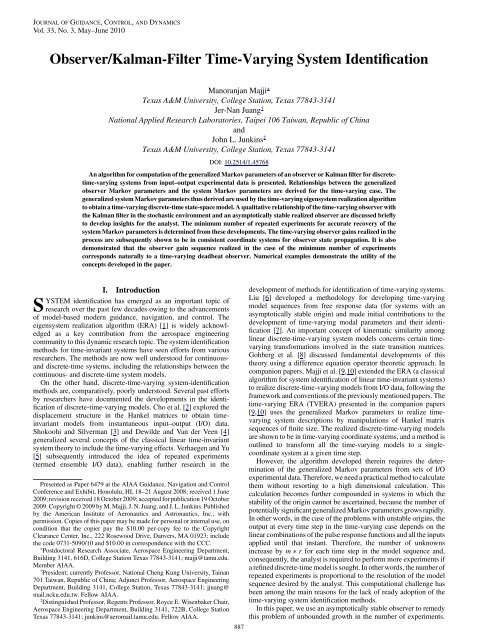
Observer/Kalman-Filter Time-Varying System Identification - AIAA

JOURNAL OF GUIDANCE,CONTROL, AND DYNAMICS 

Vol. 33, No. 3, May–June 2010 

Observer/Kalman-Filter Time-Varying System Identification 

Manoranjan Majji ∗ 

Texas A&M University, College Station, Texas 77843-3141 

Jer-Nan Juang † 

National Applied Research Laboratories, Taipei 106 Taiwan, Republic of China 

and 

John L. Junkins ‡ 

Texas A&M University, College Station, Texas 77843-3141 

DOI: 10.2514/1.45768 

An algorithm for computation of the generalized Markov parameters of an observer or Kalman filter for discretetime-varying 

systems from input–output experimental data is presented. Relationships between the generalized 

observer Markov parameters and the system Markov parameters are derived for the time-varying case. The 

generalized system Markov parameters thus derived are used by the time-varying eigensystem realization algorithm 

to obtain a time-varying discrete-time state-space model. A qualitative relationship of the time-varying observer with 

the Kalman filter in the stochastic environment and an asymptotically stable realized observer are discussed briefly 

to develop insights for the analyst. The minimum number of repeated experiments for accurate recovery of the 

system Markov parameters is determined from these developments. The time-varying observer gains realized in the 

process are subsequently shown to be in consistent coordinate systems for observer state propagation. It is also 

demonstrated that the observer gain sequence realized in the case of the minimum number of experiments 

corresponds naturally to a time-varying deadbeat observer. Numerical examples demonstrate the utility of the 

concepts developed in the paper. 

I. Introduction 

SYSTEM identification has emerged as an important topic of 

research over the past few decades owing to the advancements 

of model-based modern guidance, navigation, and control. The 

eigensystem realization algorithm (ERA) [1] is widely acknowledged 

as a key contribution from the aerospace engineering 

community to this dynamic research topic. The system identification 

methods for time-invariant systems have seen efforts from various 

researchers. The methods are now well understood for continuousand 

discrete-time systems, including the relationships between the 

continuous- and discrete-time system models. 

On the other hand, discrete-time-varying system-identification 

methods are, comparatively, poorly understood. Several past efforts 

by researchers have documented the developments in the identification 

of discrete-time-varying models. Cho et al. [2] explored the 

displacement structure in the Hankel matrices to obtain timeinvariant 

models from instantaneous input–output (I/O) data. 

Shokoohi and Silverman [3] and Dewilde and Van der Veen [4] 

generalized several concepts of the classical linear time-invariant 

system theory to include the time-varying effects. Verhaegen and Yu 

[5] subsequently introduced the idea of repeated experiments 

(termed ensemble I/O data), enabling further research in the 

Presented as Paper 6479 at the AIAA Guidance, Navigation and Control 

Conference and Exhibit, Honolulu, HI, 18–21 August 2008; received 1 June 

2009; revision received 18 October 2009; accepted for publication 19 October 

2009. Copyright © 2009 by M. Majji, J. N. Juang, and J. L. Junkins. Published 

by the American Institute of Aeronautics and Astronautics, Inc., with 

permission. Copies of this paper may be made for personal or internal use, on 

condition that the copier pay the $10.00 per-copy fee to the Copyright 

Clearance Center, Inc., 222 Rosewood Drive, Danvers, MA 01923; include 

the code 0731-5090/10 and $10.00 in correspondence with the CCC. 

∗ Postdoctoral Research Associate, Aerospace Engineering Department, 

Building 3141, 616D, College Station Texas 77843-3141; majji@tamu.edu. 

Member AIAA. 

† President; currently Professor, National Cheng Kung University, Tainan 

701 Taiwan, Republic of China; Adjunct Professor, Aerospace Engineering 

Department, Building 3141, College Station, Texas 77843-3141; jjuang@ 

mail.ncku.edu.tw. Fellow AIAA. 

‡ Distinguished Professor, Regents Professor, Royce E. Wisenbaker Chair, 

Aerospace Engineering Department, Building 3141, 722B, College Station 

Texas 77843-3141; junkins@aeromail.tamu.edu. Fellow AIAA. 

887 

development of methods for identification of time-varying systems. 

Liu [6] developed a methodology for developing time-varying 

model sequences from free response data (for systems with an 

asymptotically stable origin) and made initial contributions to the 

development of time-varying modal parameters and their identification 

[7]. An important concept of kinematic similarity among 

linear discrete-time-varying system models concerns certain timevarying 

transformations involved in the state transition matrices. 

Gohberg et al. [8] discussed fundamental developments of this 

theory using a difference equation operator theoretic approach. In 

companion papers, Majji et al. [9,10] extended the ERA (a classical 

algorithm for system identification of linear time-invariant systems) 

to realize discrete-time-varying models from I/O data, following the 

framework and conventions of the previously mentioned papers. The 

time-varying ERA (TVERA) presented in the companion papers 

[9,10] uses the generalized Markov parameters to realize timevarying 

system descriptions by manipulations of Hankel matrix 

sequences of finite size. The realized discrete-time-varying models 

are shown to be in time-varying coordinate systems, and a method is 

outlined to transform all the time-varying models to a singlecoordinate 

system at a given time step. 

However, the algorithm developed therein requires the determination 

of the generalized Markov parameters from sets of I/O 

experimental data. Therefore, we need a practical method to calculate 

them without resorting to a high dimensional calculation. This 

calculation becomes further compounded in systems in which the 

stability of the origin cannot be ascertained, because the number of 

potentially significant generalized Markov parameters grows rapidly. 

In other words, in the case of the problems with unstable origins, the 

output at every time step in the time-varying case depends on the 

linear combinations of the pulse response functions and all the inputs 

applied until that instant. Therefore, the number of unknowns 

increase by m r for each time step in the model sequence and, 

consequently, the analyst is required to perform more experiments if 

arefined discrete-time model is sought. In other words, the number of 

repeated experiments is proportional to the resolution of the model 

sequence desired by the analyst. This computational challenge has 

been among the main reasons for the lack of ready adoption of the 

time-varying system identification methods. 

In this paper, we use an asymptotically stable observer to remedy 

this problem of unbounded growth in the number of experiments.

888 MAJJI, JUANG, AND JUNKINS 

The algorithm developed as a consequence is called the time-varying 

observer/Kalman-filter system identification (TOKID). In addition, 

the tools systematically presented in this paper give an estimate 

on the minimum number of experiments needed to perform 

identification and/or recovery of all the Markov parameters of 

interest until that time instant. Thus, the central result of the current 

paper is to make the number of repeated experiments independent of 

the desired resolution of the model. Furthermore, because the 

frequency response functions for time-varying systems are not well 

known, the method outlined seems to be one of the first practical 

ways to obtain the generalized Markov parameters, bringing the 

time-varying identification methods to the table of the practicing 

engineer. 

Novel models relating I/O data are developed in this paper and are 

found to be elegant extensions of the autoregressive exogenous input 

(ARX) models, well known in the analysis of time-invariant models 

(cf., Juang et al. [11]). The ARX model is a linear difference equation 

that relates the input to the output. This generalization of the classical 

ARX model to the time-varying case admits analogous recursive 

relations with the system Markov parameters, as was developed in 

the time-invariant case. This analogy is shown to go even further and 

enable us to realize a deadbeat observer gain sequence for timevarying 

systems. The generalization of this deadbeat definition is 

rather unique and general for the time-varying systems, as it is shown 

that not all the closed-loop time-varying eigenvalues need to be zero 

for the time-varying observer gain sequence to be called deadbeat. 

Furthermore, it is demonstrated that the time-varying observer 

sequence (deadbeat or otherwise) computed from the ARX model is 

realized in a compatible coordinate system with the identified plant 

model sequence. Relations with the time-varying Kalman filter are 

made, comparing with the time-varying observer gains realized from 

the TOKID procedure presented in the paper. 

II. Basic Formulation 

We start by revisiting the relations between the I/O sets of vectors 

via the system Markov parameters, as developed in the theory 

concerning the TVERA (refer to companion paper [9], based on [10], 

and the references therein). The fundamental difference equations 

governing the evolution of a linear system in discrete time are given 

by 

together with the measurement equations: 

x k 1 A k x k B k u k (1) 

y k C k x k D k u k (2) 

with the state, output, and input dimensions x k 2 R n , y k 2 R m , and 

u k 2 R r , and the system matrices to be of compatible dimensions 

8 k 2 Z, an index set. The solution of the state evolution (the linear 

time-varying discrete-time difference equation solution) is given by 

X k 1 

x k k; k 0 x 0 k; i 1 B i u i (3) 

i k 0 

8 k k 0 1, where the state transition matrix :; : is defined as 

8 

< A k 1 ;A k 2 ; ... ;A k0 

8 k>k 0 

k; k 0 I k k 

: 

0 (4) 

undefined 8 k

MAJJI, JUANG, AND JUNKINS 889 

from experimental data. Importantly, for the first time, we are also 

able to isolate a minimum number of repeated experiments to help the 

practicing engineer plan the experiments required for identification 

a priori. 

Following the observations of the previous researchers, consider 

the use of a time-varying output–feedback-style gain sequence in the 

difference model [Eq. (1)], producing 

x k 1 A k x k B k u k G k y k G k y k 

A k G k C k x k B k G k D k u k G k y k 

" # 

A k x k B k G k D 

. u k 

k A k x k B k v k (9) 

with the definitions: 

A k A k G k C k ; B k B k G k D k G k ; v k 

u k 

y k 

(10) 

and no change in the measurement equations at the time step t k : 

G k 

y k 

y k C k x k D k u k (11) 

The outputs at the consecutive time steps, starting from the initial 

time step t 0 (denoted by k 0 0) are therefore written as 

y 0 C 0 x 0 D 0 u 0 ; 

y 1 C 1 A 0 x 0 D 1 u 1 C 1 B 0 v 0 C 1 A 0 x 0 D 0 u 0 h 1;0 v 0 ; 

y 2 C 2 A 1 A 0 x 0 D 2 u 2 C 2 B 1 v 1 C 2 A 1 B 0 v 0 

. 

C 2 A 1 A 0 x 0 D 2 u 2 h 2;1 v 1 h 2;0 v 0 ; 

(12) 

with the definition of the generalized observer Markov parameters: 

8 

< C k A k 1 ; A k 2 ; ... ; A i 1 B i 8 k>i 1 

h k;i C 

: k B k 1 k i 1 

0 8 kp), we have 

2 3 

u k 

v k 1 

y k D k h k;k 1 h k;k 2 ... h v k 2 

k;k p (17) 

6 . 7 

4 

5 

v k p 

This represents a set of m equations in m r p r m 

unknowns. In contrast to the developments using the generalized 

system Markov parameters (to relate the I/O data sets, refer to Eq. (8) 

in the companion papers [9,10] and the references therein for more 

information), the number of unknowns remains constant in this case. 

This makes the computation of observer Markov parameters possible 

in practice, because the number of repeated experiments required to 

compute these parameters is now constant (derived next) and does


not change with the discrete-time step t k . In fact, it is observed that a 

minimum of Nexp min r p r m experiments are necessary 

to determine the observer Markov parameters uniquely. From the 

developments of the subsequent sections, this is the minimum 

number of repeated experiments one should perform in order to 

realize the time-varying system models desired from the TVERA. 

Equation (17), with N repeated experiments, yields: 

Y k y 1 

k y 2 

k ... y N 

k 

2 

3 

u 1 

k u 2 

k u N 

k 

v 1 

k 1 v 2 

k 1 v N 

k 1 

D k h k;k 1 h k;k 2 ... h k;k p 

v 1 

k 2 v 2 

k 2 ... v N 

k 2 

. 

. 

. . 6 

7 

4 

5 

v 1 

k p v 2 

k p v N 

k p 

M k V k (18) 

8 k>p. Therefore, the least-squares solution for the generalized 

observer Markov parameters is given for each time step as 

^M k Y k V † k (19) 

where : † denotes the pseudoinverse of a matrix [15,16]. The 

calculation of the system Markov parameters and the observer gain 

Markov parameters is detailed in the next section. 

IV. Computation of Generalized System Markov 

Parameters and Observer Gain Sequence 

We first outline a process for the determination of a system Markov 

parameter sequence from the observer Markov parameter sequence 

calculated in the previous section. A recursive relationship is then 

given to obtain the system Markov parameters, with the index 

difference of greater than p time steps. Similar procedures are set up 

for observer gain Markov parameter sequences. 

A. Computation of System Markov Parameters from Observer 

Markov Parameters 

Considering the definition of the generalized observer Markov 

parameters, we write 

h k;k 1 C k B k 1 

C k B k 1 G k 1 D k 1 G k 1 

h 1 

k;k 1 h 2 

k;k 1 

(20) 

where the superscripts in Eqs. (1) and (2) are used to distinguish 

between the Markov parameter sequences useful to compute the 

system parameters and the observer gains, respectively. Observe the 

following manipulation, written as 

h 1 

k;k 1 h 2 

k;k 1 D k 1 C k B k 1 h k;k 1 (21) 

A similar expression for Markov parameters with two time steps 

between them yields: 

h 1 

k;k 2 

h 2 

k;k 2 D k 2 C k A k 1 B k 2 C k A k 1 G k 2 D k 2 

C k A k 1 B k 2 G k 2 D k 2 C k A k 1 G k 2 D k 2 

C k A k 1 B k 2 

C k A k 1 G k 1 C k 1 B k 2 

C k A k 1 B k 2 h 2 

k;k 1 C k 1B k 2 

h k;k 2 h 2 

k;k 1 h k 1;k 2 (22) 

This elegant manipulation leads to an expression for the system 

Markov parameter h k;k 2 to be calculated from observer Markov 

parameters at the time step t k and the system Markov parameters at 

previous time steps. This recursive relationship was found to hold in 

general and enables the calculation of the system Markov parameters 

(unadorned h i;j ) from the observer Markov parameters h i;j . 

To show this holds in general, consider the induction step 

with the observer Markov parameters (with p time-step separation) 

given by 

h 1 

k;k p h 2 

k;k p D k p C k A k 1 ; A k 2 ; ...; A k p 1 B k p G k p D k p 

C k A k 1 ; A k 2 ; ...; A k p 

C k A k 1 ; A k 2 ; ...; A k p 

1 G k p D k p 

1 B k p 

C k A k 1; A k 2 ; ...; A k p 2 A k p 1 G k p 1 C k p 1 B k p 

C k A k 1 ; A k 2 ; ...; A k p 2 ;A k p 1 B k p 

C k A k 1 ; A k 2 ; ...; A k p 2 G k p 1 C k p 1 B k p 

C k A k 1 ; A k 2 ; ...; A k p 2 A k p 1 B k p 

h 2 

k;k p 1 h k p 1;k p (23) 

Careful examination reveals that the term 

can be written as 

C k A k 1 ; A k 2 ; ... ; A k p 2 ; A k p 1 B k p 

C k A k 1 ; A k 2 ; ... ; A k p 2 ;A k p 1 B k p 

C k A k 1 ; ... ; A k p 3 A k p 2 G k p 2 C k p 2 A k p 1 B k p 

C k A k 1 ; ... ;A k p 2 ;A k p 1 B k p 

C k A k 1 ; ... ;G k p 2 C k p 2 A k p 1 B k p 

C k A k 1 ; ... ;A k p 2 ;A k p 1 B k p h 2 

k;k p 2 h k p 2;k p 

. 

C k A k 1 ; ... ;A k p 1 B k p h 2 

k;k 1 h k 1;k p 

h 2 

k;k 2 h k 2;k p h 2 


h k;k p h 2 

k;k 1 h k 1;k p h 2 

k;k 2 h k 2;k p 

h 2 

k;k p 2 h k p 2;k p (24) 

This manipulation enables us to write 

h 1 

k;k p h 2 

k;k p D k p 

h k;k p h 2 

k;k 1 h k 1;k p h 2 

k;k 2 h k 2;k p 

h k;k p 

X p 1 

h 2 


j 1 

h 2 

k;k j h k j;k p (25) 

Writing the derived relationships between the system and the 

observer Markov parameters yields the following set of equations: 

h k;k 1 h 1 

k;k 1 h 2 

k;k 1 D k 1; 

h k;k 2 h 2 

k;k 1 h k 1;k 2 h 1 

k;k 2 

h 2 

k;k 2 D k 2 

. 

h k;k p h 2 

k;k 1 h k 1;k p h 2 


h 1 

k;k p h 2 

k;k p D k p (26) 

Defining r i;j 

: h 1 

i;j h 2 

i;j D j , we obtain the system of linear 

equations, relating the system and observer Markov parameters as


2 

3 

I m h 2 

k;k 1 h 2 

k;k 2 ... h 2 

k;k p 1 

0 I m h 2 

k 1;k 2 ... h 2 

k 1;k p 2 

. . . . . 

. 6 

4 

7 

5 

0 0 0 ... I m 

2 

3 

h k;k 1 h k;k 2 ... h k;k p 

0 h k 1;k 2 ... h k 1;k p 

. . . 

. 

. 

6 

. 

7 

4 

5 

0 0 ... h k p 1;k p 

2 

3 

r k;k 1 r k;k 2 ... r k;k p 

0 r k 1;k 2 ... r k 1;k p 

. . . 

. . . 

. 

6 

. . 

7 

4 

5 

0 0 ... r k p 1;k p 

(27) 

We note the striking similarity of this equation to the relation between 

the observer Markov parameters and the system Markov parameters 

in the classical OKID algorithm for time-invariant systems (compare 

the coefficient matrix of Eq. (27) with Eq. 6.8 of Juang [1]). 

Considering the expressions for 

h k;k p 

: C k A k 1 ; ... ; A k p 1 B k p 

and choosing a p sufficiently large, we have that, owing to the 

asymptotic stability of the closed loop (including the observer), 

h k;k p 0. This fact enables us to establish recursive relationships 

for the calculation of the system Markov parameters h k;k and 

8 >p. Generalizing Eq. (25) produces: 

h k;k h 1 

k;k h 2 

k;k D k 

X 1 

j 1 

h 2 

k;k j h k j;k (28) 

for p. Then, based on the arguments involving Eq. (17) for the 

calculation of the generalized observer Markov parameters, all the 

terms with a time-step separation greater than p vanish identically, 

and we obtain the relationship: 

for 

>p. 

h k;k 

X p 

j 1 

h 2 

k;k j h k j;k (29) 

B. Computation of Observer Gain Markov Parameters from the 

Observer Markov Parameters 

Consider the generalized observer gain Markov parameters 

defined as 

h o k;i 

8 

< C k A k 1 ;A k 2 ; ... ;A i 1 G i 8 k>i 1 

C 

: k G k 1 k i 1 

0 8 kp. Therefore, to calculate the observer gain Markov 

parameters, we have a similar upper-block triangular system of linear 

equations, which can be written as 

2 

3 

I m h 2 

k;k 1 

h 2 

k;k 2 

h 2 

k;k p 1 

0 I m h 2 

k 1;k 2 

h 2 

k 1;k p 2 

. . . 

. . . 

. 

6 

4 

. 

. 

7 

5 

0 0 0 I m 

2 

3 

h o k;k 1 h o k;k 2 h o k;k p 

0 h o k 1;k 2 h o k 1;k p 

. . . 

. 

. 

6 

. 

7 

4 

5 

0 0 h o k p 1;k p 

2 

h 2 

k;k 1 h 2 

k;k 2 h 2 3 

k;k p 

0 h 2 

k 1;k 2 h 2 

k 1;k p 

. . . . . 

. (36) 

6 

7 

4 

5 

0 0 h 2 

k p 1;k p 

to be solved at each time step k. Having outlined a method to compute 

the observer gain Markov parameters, let us now proceed to look 

at the procedure to extract the observer gain sequence from them. 

C. Calculation of the Time-Varying Observer Gain Sequence 

From the definition of the observer gain Markov parameters 

[Eq. (30)], we can stack the first few parameters in a tall matrix and 

observe that


P k 1 

: 

2 

h o 3 2 

3 

k 1;k 

C k 1 G k 

h o k 2;k 

C k 2 A k 1 G k 

6 . 7 6 

. 

7 

4 . 5 4 

. 

5 

h o k m;k C k m ;A k m 1 ; ... ;A k 1 G k 

2 

3 

C k 1 

C k 2 A k 1 

6 

. 

7 

4 

5 G k O m 

k 1 G k (37) 

C k m ;A k m 1 ; ... ;A k 1 

such that a least-squares solution for the gain matrix at each time step 

is given by 

G k O m † 

k 1 P k 1 (38) 

However, from the developments of the companion paper, we find 

that it is indeed impossible to determine the observability Gramian 

in the true coordinate system [9], as suggested by Eq. (38). The 

computed observability Gramian is, in general, in a time-varying and 

unknown coordinate system denoted by O m 

k 1 at the time step t k 1. 

We will now show that the gain computed from this time-varying 

observability Gramian (computed) will be consistent with the timevarying 

coordinates of the plant model computed by the TVERA 

presented in the companion paper. Therefore, upon using the 

computed observability Gramian (in its own time-varying coordinate 

system) and proceeding with the gain calculation, as indicated by 

Eq. (38), we arrive at a consistent computed gain matrix. Given a 

transformation matrix T k 1 , 

P k 1 O m 

k 1 G k O m 

k 1 T k 1Tk 

1 

such that 

^G k Tk 

1 

1 G k 

1 G k 

Ô m 

k 1 T k 

1 

1 G k 

Ô m ^G k 1 k 

(39) 

Ô m 

k 1 † P k 1 (40) 

therefore, with no explicit intervention by the analyst, the realized 

gains are automatically in the right coordinate system for producing 

the appropriate TOKID closed loop. For consistency, it is often 

convenient if one obtains the first few time-step models, as included 

in the developments of the companion paper. This automatically 

gives the observability Gramians for the first few time steps to 

calculate the corresponding observer gain matrix values. To see that 

the gain sequence computed by the algorithm is, indeed, in consistent 

coordinate systems, recall the identified system and control influence 

and the measurement sensitivity matrices in the time-varying 

coordinate systems, to be derived as (refer to companion paper [9]) 

Â k T 1 

k 1 A kT k ; ^B k T 1 

k 1 B k; ^C k C k T k (41) 

The TOKID closed-loop system matrix, with the realized gain matrix 

sequence, is seen to be consistently given as 

V. Relationship Between the Identified Observer 

and a Kalman Filter 

We now qualitatively discuss several features of the observer, 

realized from the algorithm presented in the paper. Constructing the 

closed loop of the observer dynamics, it can be found to be 

asymptotically stable, as purported at the design stage. Following the 

developments of the time-invariant OKID paper, we use the wellunderstood 

time-varying Kalman-filter theory to make some intuitive 

observations. These observations help us address the important issue: 

variable-order GTV-ARX model fitting of I/O data and what it all 

means. Insight is also obtained as to what happens in the presence of 

measurement noise. In the practical situation, for which there is the 

presence of the process and the measurement noise in the data, the 

GTV-ARX model becomes a moving average model that can be 

termed as the GTV autoregressive moving average with exogenous 

input (GTV-ARMAX) model (generalized is used to indicate 

variable order at each time step). A detailed quantitative examination 

of this situation is beyond the scope of the current paper: the authors 

limit the discussions to qualitative relations. 

The Kalman-filter equations for a truth model given in Eq. (A1) are 

given by 

or 

^x k 1 A k ^x k B k u k (43) 

^x k 1 A k I K k C k ^x k B k u k A k K k y k (44) 

together with the propagated output equation 

^y k C k ^x k D k u k (45) 

where the gain K k is optimal [see expression in Eq. (A16)]. As 

documented in the standard estimation theory textbooks, optimality 

translates to any one of the equivalent necessary conditions of 

minimum variance, maximum likelihood, orthogonality, or Bayesian 

schemes. A brief review of the expressions for the optimal gain 

sequence is derived in the Appendix A, which also provides an 

insight into the useful notion of orthogonality of the discrete 

innovations process in addition to deriving an expression for the 

optimal gain matrix sequence [see Eq. (A16) for an expression for the 

optimal gain]. From an I/O standpoint, the innovations approach 

provides the most insight for analysis and is used in this section. 

Using the definition of the innovations process " k 

: y k ^y k , the 

measurement equation of the estimator [shown in Eq. (45)] can be 

written in favor of the system outputs, as given by 

y k C k ^x k D k u k " k (46) 

Rearranging the state propagation shown in Eq. (43), we arrive at a 

form given by 

^x k 1 A k I K k C k ^x k B k u k A k K k y k 

~A k ^x k 

~B k v k 

(47) 

Â k 

^G k ^C k T 1 

k 1 A k G k C k T k (42) 

in a kinematically similar fashion to the true TOKID closed loop. The 

nature of the computed stabilizing (deadbeat or near-deadbeat) gain 

sequence is best viewed from a reference coordinate system, as 

opposed to the time-varying coordinate systems computed by the 

algorithm. The projection-based transformations can be used for this 

purpose and are discussed in detail in the companion paper [9]. 

with the definitions 

~A k A k I K k C k ; ~B k B k A k K k ; v k 

u k 

y k 

(48) 

Notice the structural similarity in the layout of the rearranged 

equations to the TOKID equations in Sec. III. This rearrangement 

helps in making comparisons and observations as to the conditions in 

which we actually manage to obtain the Kalman-filter gain sequence 

(or otherwise). 

Starting from the initial condition, the I/O relation of the Kalmanfilter 

equations can be written as


y 0 C 0 ^x 0 D 0 u 0 " 0 ; 

y 1 C 1 

~A 0 ^x 0 D 1 u 1 C 1 

~B 0 v 0 " 1 ; 

y 2 C 2 

~A 1 

~A 0 ^x 0 D 2 u 2 C 2 

~B 1 v 1 C 2 

~A 1 

~B 0 v 0 " 2 

. 

. 

X 

y p C p 

~A p 1 ; ... ; ~A p 1 

0 ^x 0 D p u p 

~h p;p j v p j " p 

. 

. 

suggesting the general relationship 

j 1 

y k p C k p ; ~A k p 1 ; ...; ~A 0 ^x 0 D k p u k p 

kXp 1 

j 1 

(49) 

~h k p;k p j v k p j " k p (50) 

with the Kalman-filter Markov parameters ~h k;i being defined by 

8 

< C k 

~A k 1 ; ~A k 2 ; ... ; ~A i 1 

~B i 8 k>i 1 

~h o k;i C 

: k 

~B k 1 k i 1 (51) 

0 8 kp), 

if G k A k K k , together with the additional condition that " k 0 

and 8 k>p. Therefore, under these conditions, our algorithm is 

expected to produce a gain sequence that is optimal. In the presence 

of noise in the output data, the additional requirement is to satisfy the 

orthogonality (innovations property) of the residual sequence, as 

derived in Appendix A. 

However, we proceeded to enforce the p (in general p k ) term 

dependence in Eq. (16), using the additional freedom obtained 

because of the variability of the time-varying observer gains. This 

enabled us to minimize the number of repeated experiments and the 

number of computations while also arriving at the fastest observer 

gain sequence, owing to the definitions of the time-varying deadbeat 

observer notions set up in this paper (following the classical 

developments of Minamide et al. [13] and Hostetter [14], as 

discussed in Appendix B). Notice that the Kalman-filter equations 

are, in general, not truncated to the first p terms. An immediate 

question arises as to whether we can ever obtain the optimal gain 

sequence using the truncated representation for gain calculation. 

To answer this question qualitatively, we consider the I/O behavior 

of the true Kalman filter in Eq. (50). Observe that Kalman gains 

can indeed be constructed so as to obtain matching truncated 

representations of the GTV-ARX (more precisely GTV-ARMAX) 

model, as in Eq. (16), via the appropriate choice of the tuning 

parameters P 0 and Q k , for measurement and process noises. In the 

GTV-ARMAX parlance, using a lower order for p (at any given time 

step) means the incorporation of a forgetting factor, which in the 

Kalman-filter framework is tantamount to using larger values for 

the process noise parameter Q k (at the same time instant). Therefore, 

the GTV-ARX and ARMAX models used for the observer gain 

sequence and the system Markov parameter sequence in the 

algorithmic developments of this paper are intimately tied into the 

tuning parameters of the Kalman filter and represent the fundamental 

balance existing in the statistical learning theory between the 

ignorance of the model for the dynamical system and the 

incorporation of new information from the measurements. Further 

research is required to develop a more quantitative relation between 

the observer identified using the developments of the paper and the 

time-varying Kalman-filter gain sequence. 

VI. Numerical Example 

Consider the same system, as presented in an example of the 

companion paper [9]. It has an oscillatory nature and does not have a 

stable origin. In the case of the time-invariant systems, systems of 

oscillatory nature are characterized by poles on the unit circle, and the 

origin is said to be marginally stable [17,18]. However, because the 

system under consideration is not autonomous, the origin is said to be 

unstable in the sense of Lyapunov, as described in [15,19]. A separate 

classification has been provided in the theory of nonlinear systems 

for systems with an origin of this type. That is called orbital stability 

or stability, in the sense of Poincaré (cf., Meirovitch [20]). We follow 

the convention of Lyapunov and term the system under consideration 

as unstable. In this case, the plant system matrix was calculated as 

Fig. 1 

Open-loop vs TOKID closed-loop pole locations [10 repeated experiments (i.e., minimum number)]. (TV denotes time-varying.)


Fig. 2 

Error in system Markov parameters (10 repeated experiments). 

2 3 

1 0 

1 1 

A k exp A c t ; B k 

6 7 

4 0 1 5 ; 

1 0 

(52) 

with 

A c 

0 2 2 I 2 2 

K t 0 2 2 

(53) 

1 0 1 0:2 

C k 

1 1 0 0:5 ; D k 0:1 1 0 

0 1 

K t 

4 3 k 1 

1 7 3 0 k 

where the matrix is given by 

and k and 0 k are defined as k sin 10t k and 0 k : cos 10t k . The 

TOKID algorithm, as described in the main body of the paper, was 

Fig. 3 

Error in Markov parameter computations (22 repeated experiments).


applied to this example to calculate the system Markov parameters 

and the observer gain Markov parameters from the simulated 

repeated experimental data. The system Markov parameters, thus 

computed, are used by the TVERA algorithm of the companion 

paper to realize the system model sequence for all the time steps for 

which experimental data is available. We demonstrate the computation 

of the deadbeat-like observer, for which the smallest order for 

the GTV-ARX model is chosen throughout the time history of the 

identification process. Appendix B details the definition of the timevarying 

deadbeat observer for the convenience of the readers, along 

with a representative closed-loop sequence result using this example 

problem. 

In this case, we were able to realize an asymptotically stable closed 

loop for the observer equation with TOKID. In fact, two of the 

closed-loop eigenvalues could be assigned to zero. The time history 

of the open-loop and closed-loop eigenvalues, as viewed from the 

coordinate system of the initial condition response decomposition, is 

plotted in Fig. 1. 

The error incurred in the identification of the system Markov 

parameters is in two parts. The system Markov parameters for the 

significant number of steps in the GTV-ARX model are, in general, 

computed exactly. However, we would still need extra system 

Markov parameters to assemble the generalized Hankel matrix 

sequence for the TVERA algorithm. These are computed using the 

recursive relationships. The truncation of the I/O relationship with 

the observer in the loop is exact in theory. Numerical errors still play a 

role. The worst-case error, although it is sufficiently small, is incurred 

in the situation when a minimum number of experiments is performed. 

The magnitude of this error is plotted in Fig. 2 as the matrix 1 

norm of the system Markov parameter error sequence (denoted by 

k k 1 ). The comparison in this figure is made with an error in the 

system Markov parameters computed from the full I/O relationship 

without an observer. Performing a larger number of experiments, in 

general, leads to better accuracy, as shown in Fig. 3. Note that more 

experiments give a better condition number for making the 

pseudoinverse of the matrix V k , shown in Eq. (18). The accuracy is 

also improved by retaining a larger number of terms (per time step) in 

the I/O map. 

The error incurred in the system Markov parameter computation is 

directly reflected in the output error between the computed and true 

Fig. 4 

Output error comparison between true and identified plant models (10 repeated experiments). 

Fig. 5 

Output error comparison between true and identified plant models (22 repeated experiments).


Fig. 6 

Open-loop vs TOKID closed-loop state-error time history (10 repeated experiments). 

Fig. 7 

Gain history (10 repeated experiments). 

system response to the test functions. It was found to be of the same 

order of magnitude (and never greater) in several representative 

situations incorporating various test cases. The corresponding plots 

for Figs. 2 and 3 are shown in Figs. 4 and 5. 

Because the considered system is unstable (oscillatory) in nature, 

the initial condition response was used to check the nature of the 

state-error decay of the system in the presence of the identified 

observer. The open-loop response of the system (with no observer in 

the loop) and the closed-loop state-error response, including the 

realized observer, are plotted in Fig. 6. The plot represents the errors 

of convergence of a time-varying deadbeat observer to the true states 

of the system. The computed states converge to the true states in 

precisely two time steps to zero error response. The analyst should 

count the two time steps in question after the first few time steps to 

enable the unique identification of the observer gains (a total of four 

time steps for this example can be seen in the plots). This decay to 

zero was exponential and too steep to plot for the (time-varying) 

deadbeat case. However, when the order was chosen to be slightly 

higher, a near-deadbeat observer was realized. Therefore, it takes 

more than two steps for the response to decay to zero. The gain 

history of the realized observer, as seen in the initial condition 

coordinate system, is plotted as Fig. 7. 

VII. Conclusions 

This paper provides an algorithm for efficient computation of 

system Markov parameters for use in time-varying system identification. 

An observer is inserted in the I/O relations, and this leads


to effective utilization of the data in computation of the system 

Markov parameters. As a by-product, one obtains an observer gain 

sequence in the same coordinate system as the system models 

realized by the time-varying system identification algorithm. This 

observer is further found to be a time-varying deadbeat observer 

of the system. Relationship of this observer with a Kalman filter is 

detailed from an I/O standpoint. It is shown that the flexibility 

of a variable-order moving average model realized in the TOKID 

computations is related to the forgetting factor introduced by the 

process noise tuning parameter of the Kalman filter. The working of 

the algorithm is demonstrated using a simple example problem. 

Appendix A: Review of the Structure and Properties 

of the Kalman Filter 

I. Linear Estimators of the Kalman Type: Review of the Structure 

and Properties 

We review the structure and properties of the state estimators 

for linear discrete-time-varying dynamical systems (Kalman-filter 

theory [21,22]) using the innovations approach propounded by 

Kailath [23] and Mehra [24]. The most commonly used truth model 

for the linear time-varying filtering problem is given by 

x k 1 A k x k B k u k k w k (A1) 

together with the measurement equations given by 

y k C k x k D k u k k (A2) 

The process noise sequence is assumed to be a Gaussian random 

sequence with zero mean E w i 0 8 i and a variance sequence 

E w i w T j Q i ij 8 i; j, having an uncorrelated profile in time and 

no correlation with the measurement noise sequence E w i v T j 0 

8 i; j. Similarly, the measurement noise sequence is assumed to be a 

zero mean Gaussian random vector with a covariance sequence given 

by E v i v T j R i ij . The Kronecker delta is denoted as ij 0 8 i ≠ 

j and ij 1 8 i j, along with the usual notation E : for the 

expectation operator of random vectors. A typical estimator of 

the Kalman type (optimal) assumes the structure (following the 

notations of [11]): 

^x k 

^x k K k y k ^y k 

: ^x k K k " k (A3) 

where the term " k 

: y k ^y k represents the so-called innovations 

process. In classical estimation theory, this innovations process is 

defined to represent the new information brought into the estimator 

dynamics through the measurements made at each time instant. 

The state transition equations and the corresponding propagated 

measurements (most often used to compute the innovations process) 

of the estimator are given by 

^x k 1 A k ^x k B k u k A k I K k C k ^x k B k u k A k K k y k 

(A4) 

and 

^y k C k ^x k D k u k (A5) 

Defining the state estimation error to be given by e k 

: x k ^x k 

(for analysis purpose), the innovations process is related to the state 

estimation error as 

" k C k e k k (A6) 

whereas the propagation of the estimation error dynamics (estimator 

in the loop, similar to the TOKID developments of the paper) is 

governed by 

e k 1 A k I K k C k e k A k K k k k w k 

: ~A k e k A k K k k k w k (A7) 

Defining the uncertainty associated by the state estimation process, 

quantified by the covariance to be P k 

: E e k e T k , the covariance 

propagation equations are given by 

P k 1 

~A k P k 

~A T k A k K k R k K T k AT k kQ k 

T 

k (A8) 

Instead of the usual, minimum variance approach in developing the 

Kalman recursions for the discrete-time-varying linear estimator, let 

us use the orthogonality of the innovations process, a necessary 

condition for optimality and to obtain the Kalman-filter recursions. 

This property, called the innovations property, is the conceptual 

basis for projection methods [23] in a Hilbert space setting. As a 

consequence of this property, we have the following condition. 

If the gain in the observer equation is optimal, then the resulting 

recursions should render the innovations process orthogonal 

(uncorrelated) with respect to all other terms of the sequence. For any 

time step t i and a time step t i k (k>0) steps behind the ith step, we 

have that 

E " i " T i k 0 (A9) 

Using the definitions for the innovations process and the state 

estimation error, we use the relationship between them to arrive at the 

following expression for the necessary condition that 

E " i " T i k C i E e i e T i k CT i k CE e i 

T 

i k 0 (A10) 

where the two terms E v i e T i k E v i v T i k 0 drop out because of 

the lack of correlation, in lieu of the standard assumptions of the 

Kalman-filter theory. For the case of k 0, it is easy to see that 

Eq. (A10) becomes 

E " i " T i C i E e i e T i C T i E i 

T 

i C i P i C T i R i (A11) 

Applying the evolution equation for the estimation error dynamics 

for k time steps backward in time from t i , we have that 

e i 

~A i 1 ; ~A i 2 ; ... ; ~A i k 1 

~A i k e i k 

~A i 1 ; ... ; ~A i k 1 A i k K i k i k ... ~A i 1 A i 2 K i 2 i 2 

A i 1 K i 1 i 1 

~A i 1 ; ... ; ~A i k 1 i k w i k ... ~A i 1 i 2 w i 2 

i 1w i 1 

(A12) 

We obtain expressions for E e i e T i k and E e i v T i k by operating 

Eq. (A12) on both sides with e T i k and vT i k and taking the expectation 

operator 

E e i e T i k 

~A i 1 ; ~A i 2 ; ... ; ~A i k 1 

~A i k E e i k e T i k 

~A i 1 ; ~A i 2 ; ... ; ~A i k 1 

~A i k P i k (A13) 

E e i 

T 

i k 

~A i 1 ; ... ; ~A i k 1 A i k K i k E i k 

T 

i k 

~A i 1 ; ... ; ~A i k 1 A i k K i k R i k (A14) 

Substituting Eqs. (A13) and (A14) into the expression for the inner 

product shown in Eq. (A10), we arrive at the expressions for the 

Kalman gain sequence as a function of the statistics of the state 

estimation error dynamics for all time instances up to t i 1 as 

E " i " T i k C i 

~A i 1 ; ~A i 2 ; ... ; ~A i k 1 

~A i k P i k C T i k 

C i 

~A i 1 ; ... ; ~A i k 

1 A i k K i k R i k 

C i 

~A i 1 ; ~A i 2 ; ... ; ~A i k 1 

~A i k P i k C T i k A i k K i k R i k 

C i 

~A i 1 ; ~A i 2 ; ... ; ~A i k 

1 A i k P i k C T i k 

K i k R i k C i k P i k C T i k 0 (A15) 

where the definition ~A k A k I K k C k has been used to derive the 

third equality. Equation (A15) is necessary to hold for all Kalman 

type estimators with the familiar update structure, 8 k>0: 

K i k P i k C T i k R i k C i k P i k C T i k 

1 

(A16)


because of the innovations property involved. The qualitative 

relationship between the identified observer realized from the 

TOKID calculations (GTV-ARX model) and the classical Kalman 

filter is explained in the main body of the paper. 

Appendix B: Time-Varying Deadbeat Observers 

I. Time-Varying Deadbeat Observers 

It was shown in the paper that the generalization of the ARX model 

in the time-varying case gives rise to an observer that could be set to a 

deadbeat condition that has different properties and structure when 

compared with its linear time-invariant counterpart. The topic of 

extension of the deadbeat observer design to the time-varying 

systems has not been pursued aggressively in the literature, and only 

scattered results exist in this context. Minamide et. al. [13] developed 

a similar definition of the time-varying deadbeat condition and 

presented an algorithm to systematically assign the observer gain 

sequence to achieve the generalized condition thus derived. In 

contrast, through the definition of the time-varying ARX model, we 

arrive at this definition quite naturally, and we further develop plant 

models and corresponding deadbeat observer models directly from 

the I/O data. 

First, we recall the definition of a deadbeat observer in the case of 

the linear time-invariant system and present a simple example to 

illustrate the central ideas. Following the conventions of Juang [1] 

and Kailath [18], if a linear discrete-time dynamical system is 

characterized by evolution equations given by 

x k 1 Ax k Bu k (B1) 

with the measurement equations (assuming that C, A is an observable 

pair) 

y k Cx k Du k (B2) 

where the usual assumptions on the dimensionality of the state space 

are made, x k 2 R n , y k 2 R m , u k 2 R r , and C, A, and B are matrices 

of compatible dimensions. Then, the gain matrix G is said to produce 

a deadbeat observer if, and only if, the following condition is satisfied 

(the so-called deadbeat condition): 

A GC p 0 n n (B3) 

where p is the smallest integer, such that m p n and 0 n n is an 

n n matrix of zeros. 

II. Example of a Time-Invariant Deadbeat Observer 

Let us consider the following simple linear time-invariant example 

to show the ideas: 

A 

1 0 

1 2 

C 0 1 (B4) 

Now, the necessary and sufficient conditions for a deadbeat observer 

design give rise to a gain matrix: 

such that 

G 

g 1 

g 2 

A GC 2 1 g 1 g 1 3 g 2 

3 g 2 g 1 2 g 2 

2 

giving rise to the gain matrix: 

(it is easy to see that p 

verified to be given by 

G 

1 

3 

0 0 

0 0 

(B5) 

2 for this problem). The closed loop can be 

A 

GC 

1 1 

1 1 

(B6) 

which is a defective (repeated roots at the origin) and nilpotent 

matrix. Therefore, the deadbeat observer is the fastest observer that 

could possibly be achieved, because in the time-invariant case, it 

designs the observer feedback, such that the closed-loop poles are 

placed at the origin. However, it is quite interesting to note that the 

necessary conditions, albeit redundant nonlinear functions, in fact 

have a solution that exists (one typically does not have to resort to 

least-squares solutions), because some of the conditions are dependent 

on each other (not necessarily linear dependence). This nonlinear 

structure of the necessary conditions to realize a deadbeat 

observer makes the problem interesting, and several techniques are 

available to compute solutions in the time-invariant case for both 

cases when plant models are available (Minamide et al. solution [13]) 

and when only experimental data are available (OKID solution). 

Now, considering the time-varying system and following the 

notation developed in the main body of the paper, this time-varying 

deadbeat definition appears to have been naturally made. Recall 

[from Eq. (16)] that in constructing the GTV-ARX model of this 

paper, we have already used this definition. Thus, we can formally 

write the definition of a time-varying deadbeat observer as follows: 

Definition: A linear time-varying discrete-time observer is said to 

be deadbeat if there exists a gain sequence G k , such that 

A k p 1 G k p 1 C k p 1 ; A k p 2 G k p 2 C k p 2 ; 

... ; A k G k C k 0 n n (B7) 

for every k, where p is the smallest integer, such that the condition is 

satisfied. 

We now illustrate this definition using an example problem. 

III. Example of a Time-Varying Deadbeat Observer 

To show the ideas, we demonstrate the observer realized on the 

same problem used in Sec. VI of the paper and followed by a short 

discussion on the nature and properties of the time-varying deadbeat 

condition in the case of the observer design. The parameters involved 

in the example problem are given (we repeat here for convenience) as 

2 3 

1 0 

1 1 

A k exp A c t ; B k 

6 7 

4 0 1 5 ; 

1 0 

1 0 1 0:2 

C k 

1 1 0 0:5 ; D k 0:1 1 0 

0 1 

where the matrix is given by 

with 

(B8) 

A c 

0 2 2 I 2 2 

K t 0 2 2 

(B9) 

K t 

4 3 k 1 

1 7 3 0 k 

and k and k 0 are defined as k sin 10t k and k 0 : cos 10t k . 

Clearly, because m 2 and n 4 for the example, the choice of 

p 2 is made to realize the time-varying deadbeat condition. 

Considering the time step k 36 for demonstration purposes, the 

closed-loop system matrix and its eigenvalues are [where M 

denotes the vector of eigenvalues of the matrix M] computed as


2 

3 

1:5756 0:3190 0:2319 0:2779 

0:8541 0:8330 2:8982 0:0435 

A 36 G 36 C 36 6 

4 0:4961 0:0882 0:7195 0:1431 

7 

5 ; 

8:2865 1:1664 0:9282 1:6124 

2 

3 

0:1804 

0:030089 

A 36 G 36 C 36 6 

4 4:6638 33:76i 10 14 7 (B10) 

5 

4:6638 33:76i 10 14 

whereas the closed-loop system matrix (and its eigenvalues) for the 

previous time step is calculated as 

2 

3 

1:3884 0:3040 0:1597 0:2623 

0:2505 0:8103 2:7307 0:0933 

A 35 G 35 C 35 6 

4 0:4456 0:1297 0:7617 0:1265 

7 

5 ; 

7:2102 0:9015 1:5928 1:4887 

2 

3 

0:14986 

0:00093564 

A 35 G 35 C 35 6 

4 2:4455 10 11 7 

(B11) 

5 

9:2301 10 14 

For the consecutive time step, these values are found to be given by 

2 

3 

1:8156 0:3184 0:3186 0:2933 

1:3196 0:8332 2:9451 0:0113 

A 37 G 37 C 37 6 

4 0:5186 0:0855 0:7044 0:1496 

7 

5 ; 

9:7693 1:309 0:1074 1:729 

2 

3 

0:086117 

0:043863 

A 37 G 37 C 37 6 

4 1:599 10 12 7 

(B12) 

5 

2:5635 10 13 

Although clearly, each of the closed-loop member sequence A 35;36;37 

has only two zero eigenvalues (individually non-deadbeat according 

to the time-invariant definition, because all closed-loop poles are not 

placed at the origin), let us now consider the product matrices: 

A 37 G 37 C 37 A 36 G 36 C 36 

2 

0:12568 0:007105 

3 

0:01476 0:003664 

10 12 0:14537 0:019406 0:03852 0:014513 

6 

7 

4 0:07660 0:00247 0:00483 0:003081 5 

0:24691 0:26557 0:29265 0:19806 

(B13) 

and 

A 36 G 36 C 36 A 35 G 35 C 35 

2 

0:0591 0:00617 

3 

0:001388 0:005052 

10 12 0:1888 0:10671 0:098574 0:099892 

6 

7 

4 0:00311 0:021205 0:020095 0:022121 5 

0:55067 0:20917 0:15277 0:18829 

(B14) 

The examples clearly indicate that the composite transition matrices 

taken p ( 2 for this example) at a time can form a null matrix 

while still retaining nonzero eigenvalues individually. This is the 

generalization that occurs in the definition of deadbeat condition in 

the case of time-varying systems. Similar to the case of time-invariant 

systems, the observer, which is deadbeat, happens to be the fastest 

observer for the given (or realized) time-varying system model. 

We reiterate the fact that, in the current developments, the deadbeat 

observer (gain sequence) is realized naturally along with the plant 

model sequence being identified. It is not difficult to see that the 

TOKID (the GTV-ARX model construction and the deadbeat 

observer calculation) subsumes the special case when the timevarying 

discrete-time plant model is known. It is of consequence to 

observe that the procedure due to TOKID is developed directly in the 

reduced dimensional I/O space, whereas the schemes developed to 

compute the gain sequences in the paper by Minamide et al. [13], 

which is quite similar to the method outlined by Hostetter [14], are 

based on projections of the state space onto the outputs. 

Acknowledgments 

The authors wish to acknowledge the support of the Texas Institute 

of Intelligent Bio Nano Materials and Structures for Aerospace 

Vehicles funded by NASA Cooperative Agreement No. NCC-1- 

02038. Any opinions, findings, and conclusions or recommendations 

expressed in this material are those of the authors and do not 

necessarily reflect the views of NASA. 

References 

[1] Juang, J.-N., Applied System Identification, Prentice–Hall, Upper 

Saddle River, NJ, 1994, pp. 121–227. 

[2] Cho, Y. M., Xu, G., and Kailath, T., “Fast Recursive Identification of 

State Space Models via Exploitation of Displacement Structure,” 

Automatica, Vol. 30, No. 1, 1994, pp. 45–59. 

doi:10.1016/0005-1098(94)90228-3 

[3] Shokoohi, S., and Silverman, L. M., “Identification and Model 

Reduction of Time Varying Discrete Time Systems,” Automatica, 

Vol. 23, No. 4, 1987, pp. 509–521. 

doi:10.1016/0005-1098(87)90080-X 

[4] Dewilde, P., and Van der Veen, A. J., Time Varying Systems and 

Computations, Kluwer Academic, Norwell, MA, 1998, pp. 19–186. 

[5] Verhaegen, M., and Yu, X., “A Class of Subspace Model Identification 

Algorithms to Identify Periodically and Arbitrarily Time Varying 

Systems,” Automatica, Vol. 31, No. 2, 1995, pp. 201–216. 

doi:10.1016/0005-1098(94)00091-V 

[6] Liu, K., “Identification of Linear Time Varying Systems,” Journal of 

Sound and Vibration, Vol. 206, No. 4, 1997, pp. 487–505. 

doi:10.1006/jsvi.1997.1105 

[7] Liu, K., “Extension of Modal Analysis to Linear Time Varying 

Systems,” Journal of Sound and Vibration, Vol. 226, No. 1, 1999, 

pp. 149–167. 

doi:10.1006/jsvi.1999.2286 

[8] Gohberg, I., Kaashoek, M. A., and Kos, J., “Classification of Linear 

Time Varying Difference Equations Under Kinematic Similarity,” 

Integral Equations and Operator Theory, Vol. 25, No. 4, 1996, pp. 445– 

480. 

doi:10.1007/BF01203027 

[9] Majji, M., Juang, J.-N., and Junkins, J. L., “Time-Varying Eigensystem 

Realization Algorithm,” Journal of Guidance, Control, and Dynamics, 

Vol. 33, No. 1, 2010, pp. 13–28. 

doi:10.2514/1.45722 

[10] Majji, M., and Junkins, J. L., “Time Varying Eigensystem Realization 

Algorithm with Repeated Experiments,” AAS/AIAA Space Flight 

Mechanics Meeting, AIAA, Reston, VA, 2008, pp. 1069–1078; also 

American Astronomical Society Paper 08-169, 2008 

[11] Juang, J.-N., Phan, M., Horta, L., and Longman, R. W., “Identification 

of Observer/Kalman Filter Parameters: Theory and Experiments,” 

Journal of Guidance, Control, and Dynamics, Vol. 16, No. 2, 1993, 

pp. 320–329. 

doi:10.2514/3.21006 

[12] Phan, M. Q., Horta, L. G., Juang, J. N., and Longman, R. W., “Linear 

System Identification via an Asymptotically Stable Observer,” Journal 

of Optimization Theory and Applications, Vol. 79, No. 1, 1993, pp. 59– 

86. 

doi:10.1007/BF00941887 

[13] Minamide, N., Ohno, M., and Imanaka, H., “Recursive Solutions to 

Deadbeat Observers for Time Varying Multivariable Systems,” 

International Journal of Control, Vol. 45, No. 4, 1987, pp. 1311– 

1321. 

doi:10.1080/00207178708933810


[14] Hostetter, G. H., Digital Control System Design, Holt, Rinehart, and 

Winston, Philadelphia, 1988, pp. 471–539. 

[15] Junkins, J. L., and Kim, Y., Introduction to Dynamics and Control of 

Flexible Structures, AIAA, Washington, D.C., 1991, pp. 21–34. 

[16] Golub, G., and Van Loan, C. F., Matrix Computations, Johns Hopkins 

Univ. Press, Baltimore, MD, 1996, pp. 48–274. 

[17] Chen, C. T., Linear System Theory and Design, Holt, Rinehart, and 

Winston, Philadelphia, 1984, pp. 130–131. 

[18] Kailath, T., Linear Systems, Prentice–Hall, Upper Saddle River, NJ, 

1980, pp. 31–186. 

[19] Vidyasagar, M., Nonlinear Systems Analysis, 2nd ed., Society for 

Industrial and Applied Mathematics, Philadelphia, 2002. 

[20] Meirovitch, L., Elements of Vibration Analysis, McGraw–Hill, New 

York, 1986, pp. 352–353. 

[21] Kalman, R. E., and Bucy, R. S., “New Methods and Results in 

Linear Prediction and Filtering Theory,” Transactions of the ASME. 

Series D, Journal of Basic Engineering, Vol. 83, 1961, pp. 95– 

108. 

[22] Crassidis, J. L., and Junkins, J. L., Optimal Estimation of Dynamic 

Systems, CRC Press, Boca Raton, FL, 2004, pp. 243–320. 

[23] Kailath, T., “An Innovations Approach to Least-Squares Estimation 

Part 1: Linear Filtering in Additive White Noise,” IEEE Transactions on 

Automatic Control, Vol. 13, No. 6, 1968, pp. 646–655. 

doi:10.1109/TAC.1968.1099025 

[24] Mehra, R. K., “On the Identification of Variances and Adaptive Kalman 

Filtering,” IEEE Transactions on Automatic Control, Vol. 15, No. 2, 

1970, pp. 175–184. 

doi:10.1109/TAC.1970.1099422

Observer/Kalman-Filter Time-Varying System Identification - AIAA

Create successful ePaper yourself

Delete template?

Save as template?