Protocole experimental module Cristallisation Final mai-2011.pdf

1
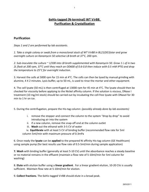
6xHis‐tagged (N‐terminal) WT VirB8.
Purification & Crystallization
Purification
Steps 1 and 2 are performed by lab assistants.
1. Take a single colony or swab from a monoclonal stock of WT VirB8 in BL21(DE3)star and grow
overnight culture on Kanamycin 50 selective LB broth at 37°C, 200 rpm.
2. Sub‐inoculate the culture ~ 1/100 into LB broth supplemented with Kanamycin 50. Grow 1 L of in two
2L flask at 200 rpm, 37°C until they reach an OD600 of 0.6‐0.8 then induce with 0.5 mM IPTG and drop
the temperature to 25°C for overnight induction.
3. Harvest the cells at 5000 rpm for 15 min at 4°C. The cells can then be lysed by manual grinding with
alumine, 4 X 2 minutes. Lysis buffer, up to 50 mL, is used to rinse the mortar and other equipment.
4. The cell lysate (50 mL) is then centrifuged at 13000 rpm for 45 min at 4°C. The lysate should then be
checked for viscosity before applying to the Nickel affinity column. If the solution is viscous, DNase I
treatment (10 mg/ml stock) should be carried out by incubating the cell‐free lysate with DNaseI for 30
min to 1 hr on ice.
5. During the centrifugation, prepare the His‐tag column: (possibly already done by lab assistants)
i. remove the stopper and connect the column to the system “drop by drop” to avoid
introducing air into the system
ii. if a new column, remove the snap‐off end at the column outlet
iii. Wash out the ethanol with 3‐5 CV of water
iv. Equilibrate with at least 5 CV of binding buffer (recommended flow rate for 5ml
column 5ml/min with maximum pressure of 0.3mPa
6. Once ready the lysate can be applied to the prepared Ni affinity His‐tag column (GE Healthcare)
using sample pump (for best results use flow rate of 0.5‐5ml/min during sample application)
7. Wash with binding buffer (generally at least 5‐10 CV) until the absorbance reaches a steady baseline
or no material remains in the effluent (maintain a flow rate of 5‐10ml/min for 5ml column for
washing)
8. Elute with elution buffer using a linear gradient. For a linear gradient elution, 10‐20 CVs is usually
sufficient. Maintain flow rate at 5‐10ml/min for elution.
9. Collect fractions. The 6xHis‐tagged VirB8 should elute in a broad peak.
26/5/2011

2
10. The protein can be dialysed versus 20 mM Tris, 200 mM NaCl (pH 7.6) and concentrated to 16‐20
mg/ml. Trays can then be set down for crystallography.
11. Regenerate the column by washing it with at least 5 CVs of binding buffer. The column is ready for
a new purification of the same protein.
Note: The column does not need to be stripped and recharged between each purification
if the same protein is to be purified. It should be sufficient to strip and recharge it after
approximately two to five purifications.
Crystallization
1. Fill the crystallization trays' wells according to the following instructions :
Salt concentration
0.775 M 0.800 M 0.825 M 0.850 M 0.875 M 0.900 M 0.925 M
1 M 20 μL 20 μL 20 μL 20 μL 20 μL 20 μL 20 μL
Na 2 HPO 4
2 M 194 μL 200 μL 206 μL 212 μL 218 μL 224 μL 230 μL
K 2 HPO 4
H 2 O 286 μL 280 μL 274 μL 268 μL 262 μL 256 μL 250 μL
Total 500 μL 500 μL 500 μL 500 μL 500μL 500 μL 500 μL
2. Form 4 uL drops on the tray's caps by mixing 2 uL of protein + 2 uL of mother liquor from the well
under standard hanging drop methods.
3. Hermetically close the wells with the caps, place the tray in a temperature‐controlled environment
(23 °C)
3. VirB8 crystals should grow within 2 days.
Stripping and Recharging the His‐tag column:
1. Strip the chromatography media by washing with at least 5 to 10 column volumes of
stripping buffer.
2. Wash with at least 5 to 10 column volumes of binding buffer.
3. Immediately wash with 5 to 10 column volumes of distilled water.
4. Recharge the water‐washed column by loading 0.5 column volumes of 0.1 M NiSO4 in
26/5/2011

3
distilled water onto the column.
5. Wash with 5 column volumes of distilled water, and 5 column volumes of binding buffer
(to adjust pH) before storage in 20% ethanol. Salts of other metals, chlorides, or sulfates
may also be used.
Note: It is important to wash with binding buffer as the last step to obtain the correct
pH before storage. Washing with buffer before applying the metal ion solution may
cause unwanted precipitation.
26/5/2011

4
6xHis-tagged (N-terminal) WT VirB8.
Crystal Mounting & Diffraction
Specialized instrumentation generating X-rays, such as generators or particles accelerators, are used to
obtain X-ray diffraction data from a crystal. The crystal is mounted for measurements so that it may be
held in the X-ray beam and rotated. A modern approach is to scoop the crystal up in a tiny loop, made
of nylon or plastic and attached to a solid rod, which is then flash-frozen with liquid nitrogen. This
freezing reduces the radiation damage caused by the X-rays. The loop is then mounted on a
goniometer, which allows it to be positioned accurately within the X-rays beam and rotated. Since both
the crystal and the beam are often very small, the crystal must be exactly centered within the beam.
Protein Crystallography deals with crystals about 0.1 mm in size and smaller; crystal mounting thus
requires very highly coordinated and precise movements and reasonable practice.
Under the microscope
1. Examine the crystallization plate under a microscope. Crystals should be the largest
possible, and have a thick, 3-dimensional rod shape.
2. Select the well giving the best looking crystals, and open it by unscrewing the cap. Place
the cap, drops up, under the microscope.
3. Using the micro-knife, remove the sticky ''skin'' covering the drops, while at the same
time try to keep the crystals from adhering to the skin. Close the cap once done.
4. Fill the aluminum bath with liquid nitrogen and put the pliers holding an empty loop
vial into the bath, allowing the vial to fill up with liquid nitrogen. Check on the liquid
nitrogen level regularly, it must always cover the vial.
5. Prepare your cryo-protection solutions in drops on a microscope glass plate, according
to the following instructions :
26/5/2011

5
Mother liquor
(μL)
Glycerol
(μL)
Total Volume
(μL)
Final
concentration (%)
Solution 1 18 2 20 10
Solution 2 16 4 20 20
Solution 3 13 7 20 35
6. Select a nylon micro-loop with an aperture that matches the size of the crystal. Use a loop
that is slightly larger than your crystal, so that the crystal doesn't rest on the edge of the loop.
7. Scoop out a crystal using the loop and plunge it into the first cryo-protection solution.
After 5 to 10 seconds, fish out your crystal and put it into the second cryo-protection
solution. Repeat for the third cryo-protection solution. The crystal will hence be plunged
into drops of progressively higher cryoprotectant concentrations.
8. Scoop out your crystal from the last drop, put the loop on the magnetic wand, and
flash-cool your crystal by putting the loop in its liquid nitrogen-filled cap. Use the magnetic
wand and leave the loop and cap in the liquid nitrogen bath.
9. Using the pliers, secure the magnetic head of the loop on the goniometer of the X-ray
generator. Remove carefully the cap with the pliers, without touching the actual loop
containing your crystal.
26/5/2011

6
On the generator
1. Check the Cryosystem first : the temperature must be 100°K.
2. On the Current board, the High Voltage must be 40 kV and the Current 25 mA. When
leaving the generator idle for extended periods of time, adjust the High Voltage to 25 kV and
the Current to 5 mA.
3. The computer controls the goniometer as well as the X-ray beam.
BCP : Crystal Centering using the goniostat
a) in Mode, select Master
b) in Tools, select Manual and then Optical
c) open up the Video
d) using the screwdriver and the A&B commands, center the beam on your crystal
e) in Manual Control, select Restore
f) Close
26/5/2011

7
APEX2 : Data collecting
a) Enter the Login and Password
b) in Open, select Protein
c) in Collect, select Experiment
leave the Hostname blank, and select Connect
d) in Setup :
i. enter the appropriate Filename
ii. enter 120 seconds under Default time
iii. enter 0.5 degrees under Default width
e) in Colones :
i. under Operation, select Phi Scan
ii. under Active, select Yes
iii. under Distance, enter 80
iv. under Theta and Omega, enter 0
v. under Phi, enter 0
.....
Fill in three lines with the exact same parameters, only modifying the Phi
value : 0, 45, and 90 degrees.
4. Manually place the detector at the 80 cm mark.
5. Open the X-rays shutter by selecting Shutter 1 Open on the dial box.
26/5/2011

8
6. Hit Execute.
7. Select Instrument and then Status to monitor the experiment.
Important Note : Use of liquid nitrogen requires certain important safety practices :
1. Always wear your lab coat, long sleeves, long trousers and closed shoes when
manipulating liquid nitrogen.
2. Always use eye goggles.
3. Always wear one pair of latex or nitrile gloves on top of a pair of white cold gloves.
4. Never operate in a closed space, as liquid nitrogen vapors can cause asphyxiation by
chasing the oxygen away.
5. Never pour liquid nitrogen in a sink or any canalization, since it can cause freezing and
breaking.
26/5/2011

9
6xHis-tagged (N-terminal) WT VirB8.
Diffraction data processing, Phasing, Refinement & Molecular Visualization
The final quality of X-Ray data is related to the data processing procedure, which includes integration
of the crystallographic data and scaling. Between experimental X-ray data and protein structure is the
structure solution procedure and phasing. Structure solution can be based on many different techniques,
depending on the data available. The next stage of protein crystallography is structure refinement, an
iterative process. Finally, protein structure representation with subsequent analysis of all features
related with this particular structure is the main goal of all protein crystallography studies.
Diffraction data processing HKL2000 ; Mosflm ; XDS
1. Reflections : when a crystal is mounted and exposed to an intense beam of X-rays, it scatters
the X-rays into a pattern of spots or reflections that can be observed and recorded. The relative
intensities of these spots provide the information to determine the arrangement of molecules
within the crystal in atomic detail.
2. High and low resolution : the peaks at small angles correspond to low-resolution data, whereas
those at high angles represent high-resolution data; thus, an upper limit on the eventual
resolution of the structure can be determined from the first few images. Some measures of
diffraction quality can be determined at this point, such as the mosaicity of the crystal and its
overall disorder, as observed in the peak widths.
3. Completeness and Symmetry : one image of spots is insufficient to reconstruct the whole
crystal; it represents only a small slice of the full Fourier transform. To collect the complete
information, the crystal must be rotated step-by-step through 180°, with an image recorded at
every step; however, if the crystal has a higher symmetry, a smaller angular range such as 90°
or 45° may be recorded.
4. Indexing : data processing begins with indexing the reflections. This means identifying the
dimensions of the unit cell and which image peak corresponds to which position in reciprocal
space. A byproduct of indexing is the determination of the symmetry of the crystal.
5. Integration : having assigned symmetry, the data is then integrated. This converts the hundreds
of images containing the thousands of reflections into a single file.
6. Merging and Scaling : a full data set may consist of hundreds of separate images taken at
different orientations of the crystal. It is essential to merge and scale these various images, that
is, to identify which peaks appear in two or more images (merging) and to scale the relative
images so that they have a consistent intensity scale (scaling).
26/5/2011

10
Phasing Experimental : SHARP ; CNS ; SOLVE ; PHASER ...
Molecular Replacement : Amore ; CNS ; Phenix ...
1. The position of each diffraction 'spot' is governed by the size and shape of the unit cell, and
the inherent symmetry within the crystal. The intensity of each diffraction 'spot' is recorded, and
this intensity is proportional to the square of the structure factor (F hkl ) amplitude. The structure
factor is a complex number containing information relating to both the amplitude and phase of a
wave. In order to obtain an interpretable electron density map ρ (x, y, z), both amplitude and
phase must be known. The phase cannot be directly recorded during a diffraction experiment:
this is known as the phase problem. Initial phase estimates can be obtained in a variety of ways,
but we will use only Molecular Replacement as part of our experiment.
2. MR tries to find the model which fits best experimental intensities among known
structures.
MR relies upon the existence of a previously solved protein structure which is homologous
(similar) to our unknown structure from which the diffraction data is derived. As for our
protein of interest VirB8, a native structure has already been deposited in the Protein Data
Bank.
i. open a web browser and go to
http://www.pdb.org/pdb/explore/explore.dostructureId=2BHM
ii. in Download Files, select PDB file (text), and save the file
iii. in the ssh window, enter kate 2BHM.pdb
iv. remove all the HETATM entries from the pdb file, and close Kate
v. we are going to use the PHENIX program to run our Molecular Replacement. In
the terminal window, enter the following command :
>phenix.refine 2BHM.pdb ...mtz strategy=rigid_body refinement.main.number_of_macro_cycles=5
prefix=ref1
vi. after a few seconds, the program abruptly stops and gives the following message :
26/5/2011

11
vii. recall the last command by using the ↑ arrow, and add the suggested command :
>phenix.refine 2BHM.pdb ...mtz strategy=rigid_body refinement.main.number_of_macro_cycles=5
prefix=ref1 ... --overwrite
Structure Refinement
CCP4 ; CNS ; Phenix ; Coot ; O
26/5/2011

12
Once an electron density map becomes available, atoms may be fitted into the map using computer
graphics to give an initial structural model of the protein. The quality of the electron density map and
structural model may be improved through iterative structural refinement, but will ultimately be limited
by the resolution of the diffraction data.
> coot &
1. when Phenix has finished, you should see ...
2. to visualize your results :
i. in the command line, enter :
ii. in Coot, select File and then Open Coordinates ...
iii. in the pop-up window, click on Filter and select ref1_001.pdb
iv. select File again, and this time click on Auto Open MTZ ...
v. in the pop-up window, click on Filter and select ref1_001_map_coeffs.mtz
vi. select Display Manager, and click on Scroll on the second line of the
pop-up window. Using the mouse scroll, adjust the FoFc map to 3.23 sigma level (upper
right-hand corner of the window). Repeat for the first line of the pop-up window,
adjusting the sigma level of the 2FoFc map to 0.91. Close the window when done.
vii. use the mouse (middle button click on selected atoms or Ctrl+right click)
to move about the structure.
viii. close Coot.
3. in the terminal window, enter
> ls
> cd ..
> mkdir ref2
> cd ref2
> cp ../ref1_001.pdb .
> cp ../ref1_001_data.mtz .
26/5/2011

13
> phenix.refine ref1_001.pdb ref1_001_data.mtz ordered_solvent=true
refinement.main.number_of_macro_cycles=5 prefix=ref2
Phenix is now using the ref1_001.pdb structure, resulting from the Molecular
Replacement phasing, and refining it against the reflection data contained in the
ref1_001_data.mtz file.
> coot
4. when Phenix is done, use Coot to visualize your newly refined structure :
i. in the command line, enter
ii. in Coot, select File and then Open Coordinates ...
iii. in the pop-up window, click on Filter and select ref2_001.pdb
iv. select File again, and this time click on Auto Open MTZ ...
v. in the pop-up window, click on Filter and select ref2_001_map_coeffs.mtz
vi. select Display Manager, and click on Scroll on the second line of the pop-up
window. Using the mouse scroll, adjust the FoFc map to 3.23 sigma level. Repeat for
the first line of the pop-up window, adjusting the sigma level of the 2FoFc map to
0.91. Close the window when done.
vii. use the mouse (click with the middle button on selected atoms or Ctrl+right
click) to move about the structure.
Note : the ordered_solvent command allowed Phenix to search and find water molecules, which are
represented as little red crosses in Coot. It is important to remember that any given protein crystal is
composed of 40 to 60 % water.
viii. close Coot.
Structural Coordinates & Molecular Visualization
O ; Coot ; PyMOL
26/5/2011

14
Once a crystal structure is determined, the information is communicated in the form of an atomic
coordinates file, that can be visualized with several programs. Molecular Visualization is the process of
interpreting visual images of molecules. You have already used Coot in order to see and modify your
protein structure as part of the refinement process; we are now going to use the PyMOL program to
better understand the aim and scope of Structural Biology.
> pymol &
1. to start PyMOL, use the command :
i. the graphic user interface (GUI) is comprised of 2 windows : the PyMOL Viewer :
and the toolbar, called the The PyMOL Molecular Graphics System
26/5/2011

15
PyMOL> load fichier.pdb
ii. to open a PDB file, you can either enter the command in PyMOL :
or click on File, Open, and select you PDB file
PyMOL> @proteinview.pml
iii. to run the visualization script prepared to help you, enter :
or click on File, Run and select proteinview.pml
iv. take a little time to play with PyMOL. You should realize that a left mouse click
allows you to turn the molecule, a right-click to zoom on it, and a middle one to center
on an atom.
v. a left-click on an atom will allow you to select a whole residue, which will then
be visible in the right hand menu as (sele), and will be highlighted in the sequence.
vi. a right-click on an atom will bring out a pop-up window
vii. to better visualize the molecule's secondary structure, click on H next to ...., and
on lines. Then, click on S and on cartoon.
2. we will now learn how to make a movie in PyMOL :
26/5/2011

16
PyMOL> reinitialize
i. re-initialize the session by entering :
or by selecting File, and Reinitialize
ii. run the visualization script again.
iii.
26/5/2011