5.2.2 Planar Andronov-Hopf bifurcation

138 CHAPTER 5. LOCAL BIFURCATION THEORY
5.2.2 Planar Andronov-Hopf bifurcation
What happens if a planar system has an equilibrium x = x 0 at some parameter
value α = α 0 with eigenvalues λ 1,2 = ±iω 0 , ω 0 > 0 (Figure 5.2(b)) Generically,
an Andronov-Hopf (or Hopf) bifurcation happens, as in the following example.
Example 5.3 (Normal form of Andronov-Hopf bifurcation)
Consider the following planar system:
{
ẋ1 = αx 1 − x 2 + sx 1 (x 2 1 + x2 2 ),
ẋ 2 = x 1 + αx 2 + sx 2 (x 2 1 + x2 2 ), (5.16)
where s = ±1. Let z = x 1 + ix 2 and ¯z = x 1 − ix 2 . Then (5.16) is equivalent to one
complex equation
ż = (α + i)z + sz 2¯z. (5.17)
Using z = ρe iϕ , one can write system (5.16) in polar coordinates:
{
˙ρ = ρ(α + sρ 2 ),
˙ϕ = 1.
(5.18)
Since the equations for ρ and ϕ are separated, one immediately gets the following
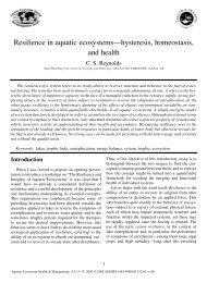
two bifurcation scenarios. If s = −1, the origin is a globally asymptotically stable
equilibrium of (5.18) for α ≤ 0. This equilibrium becomes unstable for α > 0 and
is surrounded by a stable cycle, which is a circle of radius √ α. All nonequilibrium
orbits tend to this cycle when time advances. This is a supercritical Andronov–Hopf
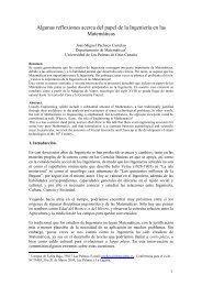
bifurcation(see Figure 5.6). If s = +1, the origin is locally acymptotically stable
Figure 5.6: Supercritical Andronov-Hopf bifurcation.
for α < 0 but is surrounded by an unstable circular cycle of radius √ −α. For
α > 0 the equilibrium at the origin becomes unstable. No cycle is present and all
nonequilibrium orbits diverge. This is a subcritical Andronov–Hopf bifurcation (see
Figure 5.7). ✸
Definition 5.4 A complex-valued function g = g(z, ¯z) is called a smooth function
of (z, ¯z) if its real and imaginary parts are smooth functions of (x 1 , x 2 ), where z =
x 1 + ix 2 .

5.2. ONE-PARAMETER LOCAL BIFURCATIONS IN ODES 139
Figure 5.7: Subcritical Andronov-Hopf bifurcation.
A smooth complex equation
ż = g(z, ¯z), z ∈ C,
is equivalent to a smooth real system
ẋ = f(x), x ∈ R 2 ,
where
x =
(
x1
x 2
)
, f(x) =
( Re[g(x1 + ix 2 , x 1 − ix 2 )]
Im[g(x 1 + ix 2 , x 1 − ix 2 )]
)
.
Definition 5.5 Two complex smooth equations are called locally topologically equivalent
near z = 0 if the corresponding planar real systems are locally topologically
equivalent near x = 0.
Local topological equivalence of parameter-dependent complex equations can be
defined similarly.
Theorem 5.4 A smooth complex equation
ż = (α + i)z + sz 2¯z + O(|z| 4 ), s = ±1, (5.19)
is locally topologically equivalent near the origin to equation (5.17).
Proof:
Step 1 (Existence and uniqueness of the cycle). Consider only the case s = −1, since
the opposite one is similar. Our first aim is to construct a Poincaré map for (5.19).
Write this equation with s = −1 in polar coordinates (ρ, ϕ):
{
˙ρ = ρ(α − ρ 2 ) + Φ(ρ, ϕ),
(5.20)
˙ϕ = 1 + Ψ(ρ, ϕ),
where Φ = O(ρ 4 ), Ψ = O(ρ 3 ), and the α-dependence of these smooth functions is
not indicated to simplify notations. An orbit of (5.20) starting at (ρ, ϕ) = (ρ 0 , 0)

140 CHAPTER 5. LOCAL BIFURCATION THEORY
ϕ
ρ1
ρ 0
ρ
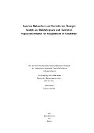
Figure 5.8: Poincaré (return) map near Hopf bifurcation.
has the following representation (see Figure 5.8): ρ = ρ(ϕ, ρ 0 ), ρ 0 = ρ(0, ρ 0 ) with ρ
satisfying the equation
dρ
dϕ = ρ(α − ρ2 ) + Φ
1 + Ψ
= ρ(α − ρ 2 ) + R(ρ, ϕ), (5.21)
where R = O(ρ 4 ). Notice that the transition from (5.20) to (5.21) is equivalent to
the introduction of a new time parametrization in which
{
˙ρ = ρ(α − ρ 2 ) + R(ρ, ϕ),
˙ϕ = 1,
In this system, the return time to the half-axis ϕ = 0 is the same for all orbits
starting on this axis with ρ 0 > 0. Since ρ(ϕ, 0) ≡ 0, we can write the Taylor
expansion for ρ(ϕ, ρ 0 ), which is a smooth function of its arguments, in the form
ρ = u 1 (ϕ)ρ 0 + u 2 (ϕ)ρ 2 0 + u 3 (ϕ)ρ 3 0 + O(|ρ 0 | 4 ). (5.22)
Substituting (5.22) into (5.21) and solving subsequently the resulting linear differential
equations at corresponding powers of ρ 0 ,
du 1
dϕ = αu 1,
du 2
dϕ = αu 2,
du 3
dϕ = αu 3 − u 3 1 ,
with the initial conditions u 1 (0) = 1, u 2 (0) = u 3 (0) = 0, we get
u 1 (ϕ) = e αϕ , u 2 (ϕ) ≡ 0, u 3 (ϕ) = 1
2α eαϕ (1 − e 2αϕ ).
Notice that these expressions are independent of the term R(ρ, ϕ). Therefore, the
Poincaré return map ρ 0 ↦→ ρ 1 = ρ(2π, ρ 0 ) has the form
ρ 1 = e 2πα ρ 0 − e 2πα [2π + O(α)]ρ 3 0 + O(ρ4 0 ) (5.23)
for all R = O(ρ 4 ). The map (5.23) can easily be analyzed for sufficiently small ρ 0
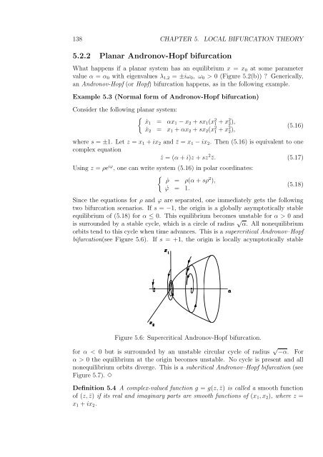
and |α|. There is a neighborhood of the origin in which the map has only a trivial
fixed point for small α < 0 and an extra fixed point, ρ (0)
0 = √ α + · · ·, for small
α > 0 (see Figure 5.9 ). The stability of the fixed points is also easily obtained from
(5.23). Taking into account that a positive fixed point of the map corresponds to a

5.2. ONE-PARAMETER LOCAL BIFURCATIONS IN ODES 141
ρ 1
α < 0
α > 0
α = 0
(0)
ρ (α)
0
ρ 0
Figure 5.9: Fixed points of the return map.
limit cycle of the system, we can conclude that system (5.20) (or equation (5.19))
with any O(|z| 4 ) terms has a unique (stable) limit cycle bifurcating from the origin
and existing for α > 0 as in equation (5.19). Therefore, in other words, higher-order
terms do not affect the limit cycle bifurcation in some neighborhood of z = 0 for |α|
sufficiently small.
Step 2 (Construction of a homeomorphism). The established existence and uniqueness
of the limit cycle is enough for all applications. Nevertheless, extra work must
be done to prove the topological equivalence of the phase portraits.
( x 1 , x 2) ( x
~
1 ,
~
x 2)
τ 0 τ 0
ρ 0 ρ 0
Figure 5.10: Construction of the homeomorphism near the Hopf bifurcation.
Fix α small but positive. The real systems corresponding to (5.17) and (5.19)
both have a unique limit cycle in some neighborhood of the origin. Assume that
the time reparametrization resulting in the constant return time 2π is performed
in (5.17) (see the previous step). Also, apply a linear scaling of the coordinates in
(5.17) such that the point of intersection of the cycle and the horizontal half-axis is
at x 1 = √ α.
Define a map z ↦→ ˜z by the following construction. Take a point z = x 1 + ix 2
and find values (ρ 0 , τ 0 ), where τ 0 is the minimal time required for an orbit of system
(5.19) to approach the point z starting from the horizontal half-axis with ρ = ρ 0 .
Now, take the point on this axis with ρ = ρ 0 and construct an orbit of (5.17) on the

142 CHAPTER 5. LOCAL BIFURCATION THEORY
time interval [0, τ 0 ] starting at this point. Denote the resulting point by ˜z = ˜x 1 +i˜x 2
(see Figure 5.10). Set ˜z = 0 for z = 0.
The map constructed is a homeomorphism that, for α > 0, maps orbits of (5.19)
in some neighborhood of the origin into orbits of (5.17) preserving time direction.
The case α < 0 can be considered in the same way without the rescaling of the
coordinates. ✷
The proof of the following theorem will occupy the rest of the Section.
Theorem 5.5 Suppose a two-dimensional system
dx
dt = f(x, α), x ∈ R2 , α ∈ R, (5.24)
with smooth f, has for all sufficiently small |α| the equilibrium x 0 (α) with eigenvalues
λ 1,2 (α) = µ(α) ± iω(α),
where µ(0) = 0, ω(0) = ω 0 > 0.
Let the following conditions be satisfied:
(B.1) l 1 (0) ≠ 0, where l 1 is the first Lyapunov coefficient;
(B.2) µ ′ (0) ≠ 0.
Then, there are invertible coordinate and parameter changes and a time reparameterization
transforming (5.24) near x 0 (α) into the system
( ) ( ) ( )
( )
d y1 β −1 y1
=
+ s(y1 2 + y 2 y1
dτ y 2 1 β y 2) + O(‖y‖ 4 ), (5.25)
2 y 2
where s = sign l 1 (0) = ±1. ✷
Remark:
One can merely say that (5.24) near (x 0 , α 0 ) is locally smoothly equivalent to
(5.25) near the origin. ♦
Since
det f x (x 0 (0), 0) = λ 1 (0)λ 2 (0) = ω 2 0 ≠ 0,
the Implicit Function Theorem guarantees the local uniqueness and smoothness of
the equilibrium x 0 (α) of (5.24) for small |α|. Shifting the origin of the coordinate
system to x 0 (α), we can then consider a smooth system
ẋ = A(α)x + F (x, α), x ∈ R 2 , α ∈ R, (5.26)
where F (x, α) = O(‖x‖ 2 ) and the matrix A(α) = f x (x 0 (α), α) has the eigenvalues
λ 1,2 (α) = µ(α) ± iω(α),
such that µ(0) = 0, ω(0) = ω 0 > 0. For small |α|,
µ(α) = 1 2 TrA(α), ω(α) = 1 2√
4 det A(α) − [TrA(α)]2 .

5.2. ONE-PARAMETER LOCAL BIFURCATIONS IN ODES 143
Lemma 5.1 Let q(α) and p(α) be smooth vector-valued functions satisfying
A(α)q(α) = λ(α)q(α), A T (α)p(α) = ¯λ(α)p(α), 〈p(α), q(α)〉 = 1,
where 〈p, q〉 ≡ ¯p T q. Introduce
z = 〈p(α), x〉 ∈ C.
Then, for sufficiently small |α|, the system (5.26) is equivalent to one complex equation:
ż = λ(α)z + g(z, ¯z, α),
where g(z, ¯z, α) = 〈p(α), F (zq(α) + ¯z¯q(α), α)〉 = O(|z| 2 ) is a smooth function of
(z, ¯z) and α.
Proof:
Let q(α) ∈ C 2 be an eigenvector of A(α) corresponding to the eigenvalue λ(α):
A(α)q(α) = λ(α)q(α),
and let p(α) ∈ C 2 be an eigenvector of the transposed matrix A T (α) corresponding
to its eigenvalue λ(α):
A T (α)p(α) = λ(α)p(α).
It is always possible to normalize p with respect to q:
〈p(α), q(α)〉 = 1,
where 〈·, ·〉 means the standard scalar product in C 2 : 〈p, q〉 = ¯p 1 q 1 + ¯p 2 q 2 . Any
vector x ∈ R 2 can be uniquely represented for any small α as
x = zq(α) + ¯z¯q(α) (3.13)
for some complex z. Indeed, we have an explicit formula to determine z:
z = 〈p(α), x〉.
To verify this formula (which results from taking the scalar product with p of both
sides of (3.13)), we have to prove that 〈p(α), ¯q(α)〉 = 0. This is the case, since
〈p, ¯q〉 = 〈p, 1¯λA¯q〉 = 1¯λ〈A T p, ¯q〉 = λ¯λ〈p, ¯q〉
and therefore (
1 − λ¯λ
)
〈p, ¯q〉 = 0.
But λ ≠ ¯λ because for all sufficiently small |α| we have ω(α) > 0. Thus, the only
possibility is 〈p, ¯q〉 = 0.
The complex variable z obviously satisfies the equation
ż = λ(α)z + 〈p(α), F (zq(α) + ¯z¯q(α), α)〉,

144 CHAPTER 5. LOCAL BIFURCATION THEORY
having the required 2 form (3.12) with
g(z, ¯z, α) = 〈p(α), F (zq(α) + ¯z¯q(α), α)〉. ✷
There is no reason to expect g to be an analytic function of z (i.e., ¯z- independent).
Write g as a formal Taylor series in two complex variables (z and ¯z):
where
g kl (α) =
for k + l ≥ 2, k, l = 0, 1, . . ..
Lemma 5.2 The equation
g(z, ¯z, α) = ∑
k+l≥2
1
k!l! g kl(α)z k¯z l ,
∂k+l
∂z k ∂¯z l 〈p(α), F (zq(α) + ¯z¯q(α), α)〉 ∣
∣∣∣z=0
,
ż = λz + g 20
2 z2 + g 11 z¯z + g 02
2 ¯z2 + O(|z| 3 ), (5.27)
where λ = λ(α) = µ(α) + iω(α), µ(0) = 0, ω(0) = ω 0 > 0, and g ij = g ij (α), can be
transformed by an invertible parameter-dependent change of complex coordinate
z = w + h 20
2 w2 + h 11 w ¯w + h 02
2 ¯w2 , (5.28)
for all sufficiently small |α|, into an equation without quadratic terms:
ẇ = λw + O(|w| 3 ).
Proof: The inverse change of variable is given by the expression
Therefore,
= λz +
w = z − h 20
2 z2 − h 11 z¯z − h 02
2 ¯z2 + O(|z| 3 ).
ẇ = ż − h 20 zż − h 11 (ż¯z + z ˙¯z) − h 02¯z ˙¯z + · · ·
( g20
)
2 − λh 20 z 2 + ( g 11 − λh 11 − ¯λh
) ( g02
11 z¯z +
2 − ¯λh
)
02 ¯z 2 + · · ·
= λw + 1 2 (g 20 − λh 20 )w 2 + (g 11 − ¯λh 11 )w ¯w + 1 2 (g 02 − (2¯λ − λ)h 02 ) ¯w 2 + O(|w| 3 ).
Thus, by setting
h 20 = g 20
λ , h 11 = g 11
¯λ , h 02 = g 02
2¯λ − λ ,
2 The vectors q(α) and p(α), corresponding to the simple eigenvalues, can be selected to depend
on α as smooth as A(α).

5.2. ONE-PARAMETER LOCAL BIFURCATIONS IN ODES 145
we “kill” all the quadratic terms in (5.27). These substitutions are correct because
the denominators are nonzero for all sufficiently small |α| since λ(0) = iω 0 with
ω 0 > 0. ✷
Remarks:
(1) The resulting coordinate transformation is polynomial with coefficients that
are smoothly dependent on α. The inverse transformation has the same property
but it is not polynomial. Its form can be obtained by the method of unknown
coefficients. In some neighborhood of the origin the transformation is near-identical
because of its linear part.
(2) Notice that the transformation changes the coefficients of the cubic (as well
as higher-order) terms of (5.27).
(3) It is instructive to compare the above given proof of Lemma 5.2 with the
corresponding proof in real notations. The equation (5.27) is equivalent to a real
system
{
ẋ1 = µx 1 − ωx 2 + 1 2 a 20x 2 1 + a 11x 1 x 2 + 1 2 a 02x 2 2 + O(‖x‖3 ),
ẋ 2 = ωx 1 + µx 2 + 1 2 b 20x 2 1 + b 11x 1 x 2 + 1 2 b 02x 2 2 + O(‖x‖3 ),
(5.29)
with µ = µ(α), ω = ω(α) as above and some smooth real functions a ij = a ij (α), b ij =
b ij (α). The transformation (5.28) becomes
{
x1 = ξ 1 + 1 2 g 20ξ 2 1 + g 11 ξ 1 ξ 2 + 1 2 g 02ξ 2 2,
x 2 = ξ 2 + 1 2 h 20ξ 2 1 + h 11 ξ 1 ξ 2 + 1 2 h 02ξ 2 2,
where g ij and h ij are unknown real finctions of α. Writing (5.29) in the (ξ 1 , ξ 2 )-
coordinates, one gets the system
⎧
⎪⎨
⎪⎩
˙ξ 1 = µξ 1 − ωξ 2 + 1(a 2 20 − µg 20 − 2ωg 11 − ωh 20 )ξ1
2
+ (a 11 + ωg 20 − µg 11 − ωg 02 − ωh 11 )ξ 1 ξ 2
+ 1(a 2 02 + 2ωg 11 − µg 02 − ωh 02 )ξ2
2
+ O(‖ξ‖ 3 ),
˙ξ 2 = ωξ 1 + µξ 2 + 1(b 2 20 + ωg 20 − µh 20 − 2ωh 11 )ξ1
2
+ (b 11 + ωg 11 + ωh 20 − µh 11 − ωh 02 )ξ 1 ξ 2
+ 1(b 2 02 + ωg 02 + 2ωh 11 − µh 02 )ξ2
2
+ O(‖ξ‖ 3 ).
(5.30)
Thus, the requirement to have no quadratic terms in this system is equivalent to
the linear algebraic system
⎛
⎜
⎝
µ 2ω 0 ω 0 0
−ω µ ω 0 ω 0
0 −2ω µ 0 0 ω
−ω 0 0 µ 2ω 0
0 −ω 0 −ω µ ω
0 0 −ω 0 −2ω µ
⎞ ⎛
⎟ ⎜
⎠ ⎝
⎞
g 20
g 11
g 02
h 20
⎟
h 11
⎠
h 02
⎛
=
⎜
⎝
a 20
a 11
a 02
b 02
b 11
b 02
⎞
. (5.31)
⎟
⎠

146 CHAPTER 5. LOCAL BIFURCATION THEORY
The matrix in the left-hand-side is nonsingular near Hopf bifurcation, since its determinant
is equal to
(9ω 2 + µ 2 )(ω 2 + µ 2 ) 2 ,
which reduces to 9ω0 6 > 0 at α = 0. Thus, for any given quadratic coefficients
a ij , b ij in (5.29), one can find from (5.31) g ij , h ij with i, j = 0, 1, 2, i + j = 2, such
that system (5.30) will have no quadratic terms for all sufficiently small |α|. This is
equivalent to Lemma 5.2. Clearly, the complex notation is simpler. ♦
Lemma 5.3 The equation
ż = λz + g 30
6 z3 + g 21
2 z2¯z + g 12
2 z¯z2 + g 03
6 ¯z3 + O(|z| 4 ),
where λ = λ(α) = µ(α) + iω(α), µ(0) = 0, ω(0) = ω 0 > 0, and g ij = g ij (α), can be
transformed by an invertible parameter-dependent change of complex coordinate
z = w + h 30
6 w3 + h 21
2 w2 ¯w + h 12
2 w ¯w2 + h 03
6 ¯w3 ,
for all sufficiently small |α|, into an equation with only one cubic term:
where c 1 = c 1 (α).
Proof:
The inverse transformation is
ẇ = λw + c 1 w 2 ¯w + O(|w| 4 ),
Therefore,
w = z − h 30
6 z3 − h 21
2 z2¯z − h 12
2 z¯z2 − h 03
6 ¯z3 + O(|z| 4 ).
ẇ = ż − h 30
2 z2 ż − h 21
2 (2z¯zż + z2 ˙¯z) − h 12
2 (ż¯z2 + 2z¯z ˙¯z) − h 03
2 ¯z2 ˙¯z + · · ·
(
g30
= λz +
6 − λh ) (
30
z 3 g21
+
2 2 − λh 21 − ¯λh )
21
z 2¯z 2
+
(
g12
2 − λh )
12
−
2
¯λh 12 z¯z 2 +
(
g03
6 − ¯λh 03
2
)
¯z 3 + · · ·
= λw + 1 6 (g 30 − 2λh 30 )w 3 + 1 2 (g 21 − (λ + ¯λ)h 21 )w 2 ¯w
+ 1 2 (g 12 − 2¯λh 12 )w ¯w 2 + 1 6 (g 03 + (λ − 3¯λ)h 03 ) ¯w 3 + O(|w| 4 ).
Thus, by setting
h 30 = g 30
2λ , h 12 = g 12
2¯λ , h 03 = g 03
3¯λ − λ ,
we can annihilate all cubic terms in the resulting equation except the w 2 ¯w -term,
which we have to treat separately. The substitutions are valid since all the involved
denominators are nonzero for all sufficiently small |α|.

5.2. ONE-PARAMETER LOCAL BIFURCATIONS IN ODES 147
One can also try to eliminate the w 2 ¯w-term by formally setting
h 21 = g 21
λ + ¯λ .
This is possible for small α ≠ 0, but the denominator vanishes at α = 0: λ(0) +
¯λ(0) = iω 0 − iω 0 = 0. To obtain a transformation that is smoothly dependent on α,
set h 21 = 0, which results in
c 1 = g 21
2 . ✷
Remarks:
(1) The remaining cubic w 2 ¯w-term is called a resonant term. Note that its
coefficient is the same as the coefficient of the cubic term z 2¯z in the original equation
in Lemma 5.3
(2) We leave to the reader a proof of Lemma 5.3 in real notations. ♦
Lemma 5.4 (Poincaré normalization) The equation
ż = λ(α)z +
∑
2≤k+l≤3
1
k!l! g kl(α)z k¯z l + O(|z| 4 ), (5.32)
where λ(α) = µ(α) + iω(α), µ(0) = 0, ω(0) = ω 0 > 0, can be transformed by an
invertible parameter-dependent change of complex coordinate, smoothly depending
on the parameter,
z = w + h 20(α)
w 2 + h 11 (α)w ¯w + h 02(α)
¯w 2
2
2
+ h 30(α)
w 3 + h 12(α)
w ¯w 2 + h 03(α)
¯w 3 + O(|w| 4 ),
6 2
6
for all sufficiently small |α|, into an equation with only one cubic term:
ẇ = λ(α)w + c 1 (α)w 2 ¯w + O(|w| 4 ), (5.33)
where
c 1 (0) =
i (
g 20 (0)g 11 (0) − 2|g 11 (0)| 2 − 1 )
2ω 0 3 |g 02(0)| 2
+ g 21(0)
. (5.34)
2
Proof: The superposition of the transformations defined by Lemmas 5.2 and 5.3
does the job. First, perform the transformation
z = w + h 20
2 w2 + h 11 w ¯w + h 02
2 ¯w2 , (5.35)
with
h 20 = g 20
λ , h 11 = g 11
¯λ , h 02 = g 02
2¯λ − λ ,
defined in Lemma 5.2. This annihilates all the quadratic terms but also changes the
coefficients of the cubic terms. The coefficient of w 2 ¯w will be 1 ˜g 2 21, say, instead of

148 CHAPTER 5. LOCAL BIFURCATION THEORY
1
g 2 21. Then make the transformation from Lemma 5.3 that eliminates all the cubic
terms but the resonant one. The coefficient of this term remains 1 ˜g 2 21.
Thus, all we need to compute, to get the coefficient c 1 in terms of the given
equation (5.32), is a new coefficient 1 ˜g 2 21 of the w 2 ¯w-term after the quadratic transformation
(5.35). For this, we can express ż in terms of w, ¯w in two ways. One way
is to substitute (5.35) into the original equation (5.32). Alternatively, since we know
the resulting form (5.33) to which (5.32) can be transformed, ż can be computed by
differentiating (5.35),
ż = ẇ + h 20 wẇ + h 11 (w ˙¯w + ¯wẇ) + h 02 ˙¯w,
and then by substituting ẇ and its complex conjugate, using (5.33). Comparing
the coefficients of the quadratic terms in the obtained expressions for ż gives the
above formulas for h 20 , h 11 , and h 02 , while equating the coefficients in front of the
w|w| 2 -term leads to
c 1 = g 20g 11 (2λ + ¯λ)
2|λ| 2 + |g 11| 2
λ + |g 02| 2
2(2λ − ¯λ) + g 21
2 .
This formula gives us the dependence of c 1 on α if we recall that λ and g ij are
smooth functions of the parameter. At the bifurcation parameter value α = 0, the
previous equation reduces to (5.34). ✷
Definition 5.6 The number
is called the first Lyapunov coefficient.
l 1 (0) = 1 ω 0
Re c 1 (0)
One has
l 1 (0) = 1
2ω 2 0
Re[ig 20 (0)g 11 (0) + ω 0 g 21 (0)]. (5.36)
Lemma 5.5 Consider the equation
dw
dt = (µ(α) + iω(α))w + c 1(α)w|w| 2 + O(|w| 4 ),
where µ(0) = 0, and ω(0) = ω 0 > 0.
Suppose µ ′ (0) ≠ 0 and l 1 (0) ≠ 0. Then, the equation can be transformed by
a parameter-dependent linear coordinate transformation, a time rescaling, and a
nonlinear time reparametrization into an equation of the form
du
dτ = (β + i)u + su|u|2 + O(|u| 4 ),
where u is a new complex coordinate, τ, β are the new time and parameter, respectively,
and s = sign l 1 (0) = ±1.