5.2.2 Planar Andronov-Hopf bifurcation

More documents

Recommendations

Info

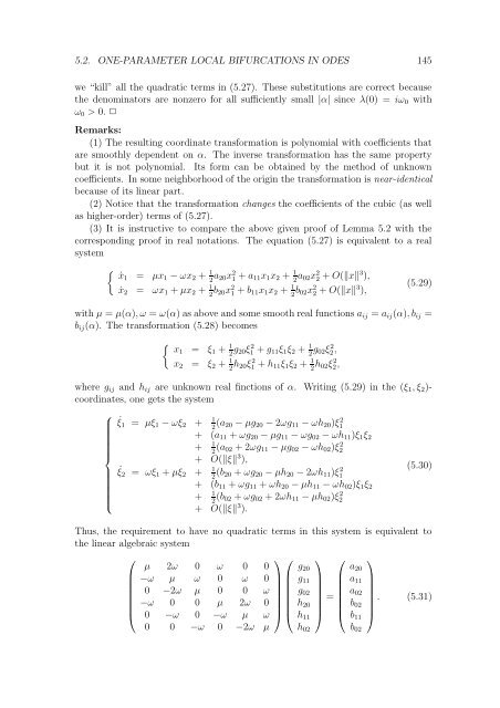
5.2. ONE-PARAMETER LOCAL BIFURCATIONS IN ODES 145 we “kill” all the quadratic terms in (5.27). These substitutions are correct because the denominators are nonzero for all sufficiently small |α| since λ(0) = iω 0 with ω 0 > 0. ✷ Remarks: (1) The resulting coordinate transformation is polynomial with coefficients that are smoothly dependent on α. The inverse transformation has the same property but it is not polynomial. Its form can be obtained by the method of unknown coefficients. In some neighborhood of the origin the transformation is near-identical because of its linear part. (2) Notice that the transformation changes the coefficients of the cubic (as well as higher-order) terms of (5.27). (3) It is instructive to compare the above given proof of Lemma 5.2 with the corresponding proof in real notations. The equation (5.27) is equivalent to a real system { ẋ1 = µx 1 − ωx 2 + 1 2 a 20x 2 1 + a 11x 1 x 2 + 1 2 a 02x 2 2 + O(‖x‖3 ), ẋ 2 = ωx 1 + µx 2 + 1 2 b 20x 2 1 + b 11x 1 x 2 + 1 2 b 02x 2 2 + O(‖x‖3 ), (5.29) with µ = µ(α), ω = ω(α) as above and some smooth real functions a ij = a ij (α), b ij = b ij (α). The transformation (5.28) becomes { x1 = ξ 1 + 1 2 g 20ξ 2 1 + g 11 ξ 1 ξ 2 + 1 2 g 02ξ 2 2, x 2 = ξ 2 + 1 2 h 20ξ 2 1 + h 11 ξ 1 ξ 2 + 1 2 h 02ξ 2 2, where g ij and h ij are unknown real finctions of α. Writing (5.29) in the (ξ 1 , ξ 2 )- coordinates, one gets the system ⎧ ⎪⎨ ⎪⎩ ˙ξ 1 = µξ 1 − ωξ 2 + 1(a 2 20 − µg 20 − 2ωg 11 − ωh 20 )ξ1 2 + (a 11 + ωg 20 − µg 11 − ωg 02 − ωh 11 )ξ 1 ξ 2 + 1(a 2 02 + 2ωg 11 − µg 02 − ωh 02 )ξ2 2 + O(‖ξ‖ 3 ), ˙ξ 2 = ωξ 1 + µξ 2 + 1(b 2 20 + ωg 20 − µh 20 − 2ωh 11 )ξ1 2 + (b 11 + ωg 11 + ωh 20 − µh 11 − ωh 02 )ξ 1 ξ 2 + 1(b 2 02 + ωg 02 + 2ωh 11 − µh 02 )ξ2 2 + O(‖ξ‖ 3 ). (5.30) Thus, the requirement to have no quadratic terms in this system is equivalent to the linear algebraic system ⎛ ⎜ ⎝ µ 2ω 0 ω 0 0 −ω µ ω 0 ω 0 0 −2ω µ 0 0 ω −ω 0 0 µ 2ω 0 0 −ω 0 −ω µ ω 0 0 −ω 0 −2ω µ ⎞ ⎛ ⎟ ⎜ ⎠ ⎝ ⎞ g 20 g 11 g 02 h 20 ⎟ h 11 ⎠ h 02 ⎛ = ⎜ ⎝ a 20 a 11 a 02 b 02 b 11 b 02 ⎞ . (5.31) ⎟ ⎠
146 CHAPTER 5. LOCAL BIFURCATION THEORY The matrix in the left-hand-side is nonsingular near <strong>Hopf</strong> <strong>bifurcation</strong>, since its determinant is equal to (9ω 2 + µ 2 )(ω 2 + µ 2 ) 2 , which reduces to 9ω0 6 > 0 at α = 0. Thus, for any given quadratic coefficients a ij , b ij in (5.29), one can find from (5.31) g ij , h ij with i, j = 0, 1, 2, i + j = 2, such that system (5.30) will have no quadratic terms for all sufficiently small |α|. This is equivalent to Lemma 5.2. Clearly, the complex notation is simpler. ♦ Lemma 5.3 The equation ż = λz + g 30 6 z3 + g 21 2 z2¯z + g 12 2 z¯z2 + g 03 6 ¯z3 + O(|z| 4 ), where λ = λ(α) = µ(α) + iω(α), µ(0) = 0, ω(0) = ω 0 > 0, and g ij = g ij (α), can be transformed by an invertible parameter-dependent change of complex coordinate z = w + h 30 6 w3 + h 21 2 w2 ¯w + h 12 2 w ¯w2 + h 03 6 ¯w3 , for all sufficiently small |α|, into an equation with only one cubic term: where c 1 = c 1 (α). Proof: The inverse transformation is ẇ = λw + c 1 w 2 ¯w + O(|w| 4 ), Therefore, w = z − h 30 6 z3 − h 21 2 z2¯z − h 12 2 z¯z2 − h 03 6 ¯z3 + O(|z| 4 ). ẇ = ż − h 30 2 z2 ż − h 21 2 (2z¯zż + z2 ˙¯z) − h 12 2 (ż¯z2 + 2z¯z ˙¯z) − h 03 2 ¯z2 ˙¯z + · · · ( g30 = λz + 6 − λh ) ( 30 z 3 g21 + 2 2 − λh 21 − ¯λh ) 21 z 2¯z 2 + ( g12 2 − λh ) 12 − 2 ¯λh 12 z¯z 2 + ( g03 6 − ¯λh 03 2 ) ¯z 3 + · · · = λw + 1 6 (g 30 − 2λh 30 )w 3 + 1 2 (g 21 − (λ + ¯λ)h 21 )w 2 ¯w + 1 2 (g 12 − 2¯λh 12 )w ¯w 2 + 1 6 (g 03 + (λ − 3¯λ)h 03 ) ¯w 3 + O(|w| 4 ). Thus, by setting h 30 = g 30 2λ , h 12 = g 12 2¯λ , h 03 = g 03 3¯λ − λ , we can annihilate all cubic terms in the resulting equation except the w 2 ¯w -term, which we have to treat separately. The substitutions are valid since all the involved denominators are nonzero for all sufficiently small |α|.
Page 1 and 2: 138 CHAPTER 5. LOCAL BIFURCATION TH
Page 7: 144 CHAPTER 5. LOCAL BIFURCATION TH
Page 11: 148 CHAPTER 5. LOCAL BIFURCATION TH

5.2.2 Planar Andronov-Hopf bifurcation

Create successful ePaper yourself

Delete template?

Save as template?