5.2.2 Planar Andronov-Hopf bifurcation

More documents

Recommendations

Info

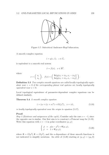
5.2. ONE-PARAMETER LOCAL BIFURCATIONS IN ODES 139 Figure 5.7: Subcritical Andronov-Hopf bifurcation. A smooth complex equation ż = g(z, ¯z), z ∈ C, is equivalent to a smooth real system ẋ = f(x), x ∈ R 2 , where x = ( x1 x 2 ) , f(x) = ( Re[g(x1 + ix 2 , x 1 − ix 2 )] Im[g(x 1 + ix 2 , x 1 − ix 2 )] ) . Definition 5.5 Two complex smooth equations are called locally topologically equivalent near z = 0 if the corresponding planar real systems are locally topologically equivalent near x = 0. Local topological equivalence of parameter-dependent complex equations can be defined similarly. Theorem 5.4 A smooth complex equation ż = (α + i)z + sz 2¯z + O(|z| 4 ), s = ±1, (5.19) is locally topologically equivalent near the origin to equation (5.17). Proof: Step 1 (Existence and uniqueness of the cycle). Consider only the case s = −1, since the opposite one is similar. Our first aim is to construct a Poincaré map for (5.19). Write this equation with s = −1 in polar coordinates (ρ, ϕ): { ˙ρ = ρ(α − ρ 2 ) + Φ(ρ, ϕ), (5.20) ˙ϕ = 1 + Ψ(ρ, ϕ), where Φ = O(ρ 4 ), Ψ = O(ρ 3 ), and the α-dependence of these smooth functions is not indicated to simplify notations. An orbit of (5.20) starting at (ρ, ϕ) = (ρ 0 , 0)
140 CHAPTER 5. LOCAL BIFURCATION THEORY ϕ ρ1 ρ 0 ρ Figure 5.8: Poincaré (return) map near Hopf bifurcation. has the following representation (see Figure 5.8): ρ = ρ(ϕ, ρ 0 ), ρ 0 = ρ(0, ρ 0 ) with ρ satisfying the equation dρ dϕ = ρ(α − ρ2 ) + Φ 1 + Ψ = ρ(α − ρ 2 ) + R(ρ, ϕ), (5.21) where R = O(ρ 4 ). Notice that the transition from (5.20) to (5.21) is equivalent to the introduction of a new time parametrization in which { ˙ρ = ρ(α − ρ 2 ) + R(ρ, ϕ), ˙ϕ = 1, In this system, the return time to the half-axis ϕ = 0 is the same for all orbits starting on this axis with ρ 0 > 0. Since ρ(ϕ, 0) ≡ 0, we can write the Taylor expansion for ρ(ϕ, ρ 0 ), which is a smooth function of its arguments, in the form ρ = u 1 (ϕ)ρ 0 + u 2 (ϕ)ρ 2 0 + u 3 (ϕ)ρ 3 0 + O(|ρ 0 | 4 ). (5.22) Substituting (5.22) into (5.21) and solving subsequently the resulting linear differential equations at corresponding powers of ρ 0 , du 1 dϕ = αu 1, du 2 dϕ = αu 2, du 3 dϕ = αu 3 − u 3 1 , with the initial conditions u 1 (0) = 1, u 2 (0) = u 3 (0) = 0, we get u 1 (ϕ) = e αϕ , u 2 (ϕ) ≡ 0, u 3 (ϕ) = 1 2α eαϕ (1 − e 2αϕ ). Notice that these expressions are independent of the term R(ρ, ϕ). Therefore, the Poincaré return map ρ 0 ↦→ ρ 1 = ρ(2π, ρ 0 ) has the form ρ 1 = e 2πα ρ 0 − e 2πα [2π + O(α)]ρ 3 0 + O(ρ4 0 ) (5.23) for all R = O(ρ 4 ). The map (5.23) can easily be analyzed for sufficiently small ρ 0 and |α|. There is a neighborhood of the origin in which the map has only a trivial fixed point for small α < 0 and an extra fixed point, ρ (0) 0 = √ α + · · ·, for small α > 0 (see Figure 5.9 ). The stability of the fixed points is also easily obtained from (5.23). Taking into account that a positive fixed point of the map corresponds to a
Page 1: 138 CHAPTER 5. LOCAL BIFURCATION TH
Page 5 and 6: 142 CHAPTER 5. LOCAL BIFURCATION TH
Page 11: 148 CHAPTER 5. LOCAL BIFURCATION TH

5.2.2 Planar Andronov-Hopf bifurcation

Create successful ePaper yourself

Delete template?

Save as template?