- Page 2 and 3:
This page intentionally left blank
- Page 5 and 6:
CRYSTALLIZATION OF POLYMERS SECOND
- Page 7:
To Berdie, my wife, and to my grand
- Page 10 and 11:
viii Contents 4.3 Two chemically id
- Page 12 and 13:
x Preface to second edition of both
- Page 14 and 15:
xii Preface to first edition of the
- Page 17 and 18:
1 Introduction 1.1 Background Polym
- Page 19 and 20:
1.2 Structure of disordered chains
- Page 21 and 22:
1.2 Structure of disordered chains
- Page 23 and 24:
1.2 Structure of disordered chains
- Page 25 and 26:
1.3 The ordered polymer chain 9 Tab
- Page 27 and 28:
1.3 The ordered polymer chain 11 Fi
- Page 29 and 30:
1.3 The ordered polymer chain 13 Fi
- Page 31 and 32:
1.4 Morphological features 15 Fig.
- Page 33 and 34:
1.4 Morphological features 17 (a) (
- Page 35 and 36:
1.4 Morphological features 19 Fig.
- Page 37 and 38:
1.4 Morphological features 21 Fig.
- Page 39 and 40:
References 23 5. Wilson, E. B., Jr.
- Page 41 and 42:
2.1 Introduction 25 Fig. 2.1 Fusion
- Page 43 and 44:
2.2 Nature of the fusion process 27
- Page 45 and 46:
2.2 Nature of the fusion process 29
- Page 47 and 48:
2.2 Nature of the fusion process 31
- Page 49 and 50:
2.2 Nature of the fusion process 33
- Page 51 and 52:
2.3 Fusion of the n-alkanes and oth
- Page 53 and 54:
2.3 Fusion of the n-alkanes and oth
- Page 55 and 56:
2.3 Fusion of the n-alkanes and oth
- Page 57 and 58:
2.3 Fusion of the n-alkanes and oth
- Page 59 and 60:
2.3 Fusion of the n-alkanes and oth
- Page 61 and 62:
2.3 Fusion of the n-alkanes and oth
- Page 63 and 64:
2.3 Fusion of the n-alkanes and oth
- Page 65 and 66:
2.4 Polymer equilibrium 49 Fig. 2.1
- Page 67 and 68:
2.4 Polymer equilibrium 51 Fig. 2.8
- Page 69 and 70:
2.4 Polymer equilibrium 53 defined
- Page 71 and 72:
with ζ e being defined as 2σ eq =
- Page 73 and 74:
2.4 Polymer equilibrium 57 is thus
- Page 75 and 76:
2.4 Polymer equilibrium 59 The data
- Page 77 and 78:
2.4 Polymer equilibrium 61 crystall
- Page 79 and 80:
2.4 Polymer equilibrium 63 Fig. 2.2
- Page 81 and 82:
2.5 Nonequilibrium states 65 Fig. 2
- Page 83 and 84:
References 67 as do low molecular w
- Page 85 and 86:
References 69 56. Beech, D. R., C.
- Page 87 and 88:
3.2 Melting temperature 71 and ζ =
- Page 89 and 90:
3.2 Melting temperature 73 1.05 1.0
- Page 91 and 92:
3.2 Melting temperature 75 140 135
- Page 93 and 94:
3.2 Melting temperature 77 Fig. 3.4
- Page 95 and 96:
3.2 Melting temperature 79 Table 3.
- Page 97 and 98:
3.2 Melting temperature 81 crystall
- Page 99 and 100: 3.2 Melting temperature 83 Fig. 3.9
- Page 101 and 102: 3.2 Melting temperature 85 Fig. 3.1
- Page 103 and 104: 3.3 Crystallization from dilute sol
- Page 105 and 106: 3.3 Crystallization from dilute sol
- Page 107 and 108: 3.3 Crystallization from dilute sol
- Page 109 and 110: 3.3 Crystallization from dilute sol
- Page 111 and 112: 3.3 Crystallization from dilute sol
- Page 113 and 114: 3.4 Helix-coil transition 97 primar
- Page 115 and 116: 3.4 Helix-coil transition 99 transi
- Page 117 and 118: 3.4 Helix-coil transition 101 If wi
- Page 119 and 120: 3.5 Transformations without change
- Page 121 and 122: 3.5 Transformations without change
- Page 123 and 124: 3.5 Transformations without change
- Page 125 and 126: 3.5 Transformations without change
- Page 127 and 128: 3.6 Chemical reactions: melting and
- Page 129 and 130: 3.6 Chemical reactions: melting and
- Page 131 and 132: 3.6 Chemical reactions: melting and
- Page 133 and 134: References 117 Fig. 3.28 Phase diag
- Page 135 and 136: References 119 45. Sanchez, I. C. a
- Page 137 and 138: References 121 121. Paternostre, L.
- Page 139 and 140: 4.2 Homogeneous melt: background 12
- Page 141 and 142: 4.2 Homogeneous melt: background 12
- Page 143 and 144: 4.2 Homogeneous melt: background 12
- Page 145 and 146: 4.2 Homogeneous melt: background 12
- Page 147 and 148: 4.2 Homogeneous melt: background 13
- Page 149: 4.3 Two chemically identical polyme
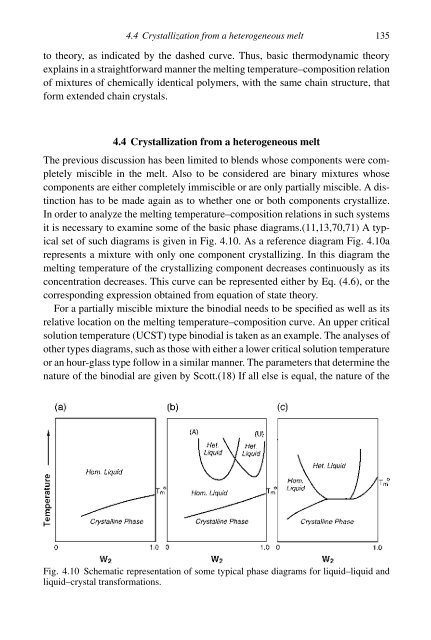
- Page 153 and 154: 4.4 Crystallization from a heteroge
- Page 155 and 156: References 139 20. Flory, P. J., Di
- Page 157 and 158: 5 Fusion of copolymers 5.1 Introduc
- Page 159 and 160: 5.2 Equilibrium theory 143 distribu
- Page 161 and 162: 5.2 Equilibrium theory 145 Here G
- Page 163 and 164: 5.2 Equilibrium theory 147 Fig. 5.1
- Page 165 and 166: Therefore 5.2 Equilibrium theory 14
- Page 167 and 168: 5.2 Equilibrium theory 151 effect o
- Page 169 and 170: 5.2 Equilibrium theory 153 would be
- Page 171 and 172: 5.3 Nonequilibrium considerations 1
- Page 173 and 174: 5.4 Experimental results: random ty
- Page 175 and 176: 5.4 Experimental results: random ty
- Page 177 and 178: 5.4 Experimental results: random ty
- Page 179 and 180: 5.4 Experimental results: random ty
- Page 181 and 182: 5.4 Experimental results: random ty
- Page 183 and 184: 5.4 Experimental results: random ty
- Page 185 and 186: 5.4 Experimental results: random ty
- Page 187 and 188: 5.4 Experimental results: random ty
- Page 189 and 190: 5.4 Experimental results: random ty
- Page 191 and 192: 5.4 Experimental results: random ty
- Page 193 and 194: 5.4 Experimental results: random ty
- Page 195 and 196: 5.4 Experimental results: random ty
- Page 197 and 198: 5.4 Experimental results: random ty
- Page 199 and 200: 5.4 Experimental results: random ty
- Page 201 and 202:
5.4 Experimental results: random ty
- Page 203 and 204:
5.4 Experimental results: random ty
- Page 205 and 206:
5.4 Experimental results: random ty
- Page 207 and 208:
5.4 Experimental results: random ty
- Page 209 and 210:
5.5 Branching 193 with 1,3-dioxolan
- Page 211 and 212:
5.6 Alternating copolymers 195 Mult
- Page 213 and 214:
5.6 Alternating copolymers 197 Fig.
- Page 215 and 216:
5.6 Alternating copolymers 199 Pair
- Page 217 and 218:
5.7 Block or ordered copolymers 201
- Page 219 and 220:
5.7 Block or ordered copolymers 203
- Page 221 and 222:
5.7 Block or ordered copolymers 205
- Page 223 and 224:
5.7 Block or ordered copolymers 207
- Page 225 and 226:
5.7 Block or ordered copolymers 209
- Page 227 and 228:
5.7 Block or ordered copolymers 211
- Page 229 and 230:
5.7 Block or ordered copolymers 213
- Page 231 and 232:
5.7 Block or ordered copolymers 215
- Page 233 and 234:
5.7 Block or ordered copolymers 217
- Page 235 and 236:
5.7 Block or ordered copolymers 219
- Page 237 and 238:
5.7 Block or ordered copolymers 221
- Page 239 and 240:
5.7 Block or ordered copolymers 223
- Page 241 and 242:
5.8 Copolymer-diluent mixtures 225
- Page 243 and 244:
References 227 are interconnected b
- Page 245 and 246:
References 229 57. Etlis, V. S., K.
- Page 247 and 248:
References 231 125. Montaudo, G., G
- Page 249 and 250:
References 233 193. Hamley, I. W.,
- Page 251 and 252:
References 235 267. Inoue, T., H. K
- Page 253 and 254:
6.2 Melting temperatures, heats and
- Page 255 and 256:
Table 6.1. Thermodynamic quantities
- Page 257 and 258:
acrylonitrile 593.2 5 021 94.7 8.5
- Page 259 and 260:
trans-octenamer 5 350.2 23 765 215.
- Page 261 and 262:
3-ethyl 3-methyl oxetane 334.2 6 27
- Page 263 and 264:
decamethylene adipate 352.7 42 677
- Page 265 and 266:
β-propiolactone 357 8 577 119.1 24
- Page 267 and 268:
caprolactam γ 7 502.2 17 949 158.8
- Page 269 and 270:
tetramethyl-p-silphenylene siloxane
- Page 271 and 272:
11 The value of H u was determined
- Page 273 and 274:
uu. Rijke, A. M. and S. McCoy, J. P
- Page 275 and 276:
Table 6.2. Thermodynamic quantities
- Page 277 and 278:
ethylene suberate 336.2 24 451 131.
- Page 279 and 280:
1 Adapted with permission from L. M
- Page 281 and 282:
Table 6.3. Unique values of thermod
- Page 283 and 284:
3,3 ′ -dimethyl thietane 286.2 5
- Page 285 and 286:
undecane amide 514.2 35 982 196.6 7
- Page 287 and 288:
new-TPI 12 >679.2 63 800 116 93.9 D
- Page 289 and 290:
i. Wrasidlo, W., J. Polym. Sci.: Po
- Page 291 and 292:
6.2 Melting temperatures, heats and
- Page 293 and 294:
6.2 Melting temperatures, heats and
- Page 295 and 296:
6.2 Melting temperatures, heats and
- Page 297 and 298:
6.2 Melting temperatures, heats and
- Page 299 and 300:
6.2 Melting temperatures, heats and
- Page 301 and 302:
6.2 Melting temperatures, heats and
- Page 303 and 304:
6.2 Melting temperatures, heats and
- Page 305 and 306:
6.2 Melting temperatures, heats and
- Page 307 and 308:
6.2 Melting temperatures, heats and
- Page 309 and 310:
6.2 Melting temperatures, heats and
- Page 311 and 312:
6.2 Melting temperatures, heats and
- Page 313 and 314:
6.2 Melting temperatures, heats and
- Page 315 and 316:
6.2 Melting temperatures, heats and
- Page 317 and 318:
6.2 Melting temperatures, heats and
- Page 319 and 320:
6.2 Melting temperatures, heats and
- Page 321 and 322:
6.2 Melting temperatures, heats and
- Page 323 and 324:
6.2 Melting temperatures, heats and
- Page 325 and 326:
6.2 Melting temperatures, heats and
- Page 327 and 328:
6.3 Entropy of fusion 311 regularit
- Page 329 and 330:
6.3 Entropy of fusion 313 Fig. 6.12
- Page 331 and 332:
6.3 Entropy of fusion 315 Table 6.5
- Page 333 and 334:
6.3 Entropy of fusion 317 disordere
- Page 335 and 336:
6.4 Polymorphism 319 of chains.(219
- Page 337 and 338:
6.4 Polymorphism 321 different crys
- Page 339 and 340:
6.4 Polymorphism 323 at 5 kbar. The
- Page 341 and 342:
6.4 Polymorphism 325 the conversion
- Page 343 and 344:
References 327 Fig. 6.16 Schematic
- Page 345 and 346:
References 329 43. Miller, R. G. J.
- Page 347 and 348:
References 331 114. Allen, G., C. B
- Page 349 and 350:
References 333 182. Russell, T. P.,
- Page 351 and 352:
References 335 256. Vogelsong, D. C
- Page 353 and 354:
7 Fusion of cross-linked polymers 7
- Page 355 and 356:
7.2 Theory of the melting of isotro
- Page 357 and 358:
7.2 Theory of the melting of isotro
- Page 359 and 360:
7.3 Melting temperature for random
- Page 361 and 362:
7.3 Melting temperature for random
- Page 363 and 364:
7.4 Melting temperature for axially
- Page 365 and 366:
7.5 Melting temperature for randoml
- Page 367 and 368:
7.6 Melting of network-diluent mixt
- Page 369 and 370:
7.6 Melting of network-diluent mixt
- Page 371 and 372:
References 355 if the cross-linkage
- Page 373 and 374:
8 Oriented crystallization and cont
- Page 375 and 376:
8.1 Introduction 359 disordered cha
- Page 377 and 378:
8.2 One-component system subject to
- Page 379 and 380:
8.2 One-component system subject to
- Page 381 and 382:
8.2 One-component system subject to
- Page 383 and 384:
8.2 One-component system subject to
- Page 385 and 386:
8.2 One-component system subject to
- Page 387 and 388:
8.2 One-component system subject to
- Page 389 and 390:
8.2 One-component system subject to
- Page 391 and 392:
8.2 One-component system subject to
- Page 393 and 394:
8.2 One-component system subject to
- Page 395 and 396:
8.2 One-component system subject to
- Page 397 and 398:
8.3 Multicomponent systems subject
- Page 399 and 400:
8.3 Multicomponent systems subject
- Page 401 and 402:
8.3 Multicomponent systems subject
- Page 403 and 404:
8.3 Multicomponent systems subject
- Page 405 and 406:
8.4 In the absence of tension 389 8
- Page 407 and 408:
8.4 In the absence of tension 391 F
- Page 409 and 410:
8.4 In the absence of tension 393 o
- Page 411 and 412:
8.5 Contractility in the fibrous pr
- Page 413 and 414:
8.5 Contractility in the fibrous pr
- Page 415 and 416:
8.5 Contractility in the fibrous pr
- Page 417 and 418:
8.5 Contractility in the fibrous pr
- Page 419 and 420:
8.6 Mechanochemistry 403 The curve
- Page 421 and 422:
8.6 Mechanochemistry 405 Fig. 8.20
- Page 423 and 424:
8.6 Mechanochemistry 407 For exampl
- Page 425 and 426:
References 409 33. Ronca, G. and G.
- Page 427 and 428:
Author index Numbers in parentheses
- Page 429 and 430:
Author index 413 Cella, R.J., 219,
- Page 431 and 432:
Author index 415 Fujii, K., 256, 32
- Page 433 and 434:
Author index 417 Jakeways, R., 335
- Page 435 and 436:
Author index 419 Marchessault, R.H.
- Page 437 and 438:
Author index 421 Porri, L., 329, 33
- Page 439 and 440:
Author index 423 Stehling, F.C., 14
- Page 441 and 442:
Author index 425 Wittner, H., 232 W
- Page 443 and 444:
Subject index 427 comonomers, 152-4
- Page 445 and 446:
Subject index 429 poly(1,4-butylene
- Page 447 and 448:
Subject index 431 poly(1,4-isoprene
- Page 449:
Subject index 433 rubber enthalpy o