Feature Preserving Mesh Simplification Using Feature Sensitive Metric
Feature Preserving Mesh Simplification Using Feature Sensitive Metric
Feature Preserving Mesh Simplification Using Feature Sensitive Metric

You also want an ePaper? Increase the reach of your titles
YUMPU automatically turns print PDFs into web optimized ePapers that Google loves.
598 J. Comput. Sci. & Technol., May 2010, Vol.25, No.3<br />
about feature line [8] . This may cause some singular<br />
problem during the process because they have identical<br />
position vector in R 3 . The treatments for blow-up<br />
region are discussed in Section 4.<br />
3.2 Derive Quadric Matrix in FS Space<br />
Definition of the cost function is a pacing factor for<br />
visual effect. It is noticed that a mesh in FS space is actually<br />
a 2-manifold embed in R 6 . FS space is therefore<br />
a non-free form space that is constrained by the geometric<br />
properties and topology in three-dimensional<br />
Euclidian space. Because the input model is existing in<br />
R 3 in essence, operations in FS space must satisfy the<br />
space restriction. Error measurements is then defined<br />
from R 6 to original R 3 . Previous works have chosen to<br />
use the discrete approximation of the tangent plane at<br />
a mesh vertex. Here we map the planes of the triangles<br />
that meet at the original vertex in R 3 onto a 2-d hyperplane<br />
embed in R 6 to approximate the corresponding<br />
tangent space. The contraction cost is then defined by<br />
the squared distance between the space point and that<br />
2-d hyperplane.<br />
As we have three given points lying on the triangle<br />
that are mapped from R 3 , one can always get two edge<br />
vectors e 1 and e 2 in R 6 . Then, for a six-dimensional<br />
element v, evaluating the distance to the 2-hyperplane<br />
which determined by this triangle is essentially equivalent<br />
to finding the nearest point v min in the linear<br />
subspace W that is spanned by e 1 and e 2 :<br />
d 2 i = min‖v − v t ‖ 2 , v t ∈ W (2)<br />
The squared distance from an arbitrary vertex v in FS<br />
space to the subspace W is now established as:<br />
d 2 i = v 2 ⊥<br />
= (v − v i ) T K T K(v − v i )<br />
= (v − v i ) T K(v − v i ). (7)<br />
Thus the error metric for v i can be easily derived in an<br />
additional form:<br />
ε i (v) = ∑ d 2 i<br />
= ∑ (v − v i ) T K i (v − v i )<br />
= (v − v i ) T ∑ K i (v − v i )<br />
= (v − v i ) T Q i (v − v i ) (8)<br />
where Q i is set to be the error matrix of v i . Similar to<br />
the previous works, we suggest using homogenous form<br />
to represent ε i , thus the updated error of new contract<br />
point can simply become an additional form.<br />
3.3 Contraction Point Optimization<br />
Edge contraction can be treated as an iteration process.<br />
Although we can simply choose the target position<br />
as v i , v j or their midpoint, to preserve geometric details<br />
as much as possible, the best choice is to estimate an<br />
optimized location that minimizes the six-dimensional<br />
quadric error with the geometric constraint in R 3 .<br />
where v t is an arbitrary vertex in W . To this end, we<br />
aimed to finding a vector v ⊥ = v − v min − v i which<br />
is orthogonal to the linear subspace W with its origin<br />
at v i . Let us define a 2 × 6 matrix A = [e 1 e 2 ] T and<br />
local coordinates x min on the basis of the subspace, i.e.,<br />
v min = A T x min + v i . We could now set an equation as:<br />
A(v − A T x min − v i ) = 0. (3)<br />
Solving (3) w.r.t. x min , we derived that<br />
So that<br />
v min = A T (AA T ) −1 A(v − v i ). (4)<br />
v ⊥ = v − v min − v i<br />
= (I − A T (AA T ) −1 A)(v − v i )<br />
= K(v − v i ). (5)<br />
Obviously, K is a 6 × 6 symmetric matrix. Moreover,<br />
we also noticed that K is implicitly comprised of the<br />
Moore-Penrose inversion of A. Therefore, K can be<br />
rewritten as K = I − A + A, such a matrix is idempotent:<br />
K 2 = K T K = K. (6)<br />
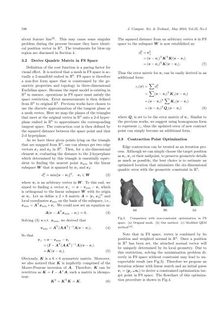
Fig.3.<br />
Comparison with non-constraint optimization in FS<br />
space. (a) Original mesh. (b) Our method. (c) Modified QEM<br />
method [12] .<br />
Note that in FS space, vertex is combined by its<br />
position and weighted normal in R 3 . Once a position<br />
in R 3 has been set, the attached normal vector will<br />
be uniquely determined by its local geometry. Due to<br />
this restriction, solving the minimization problem directly<br />
in FS space without constraint may lead to unexpectable<br />
result (see Fig.3). Therefore we propose an<br />
iteration scheme with linear search and an initial guess<br />
v i = (p i , ωn i ) to derive a constrained optimization target<br />
point in FS space. The flowchart of this optimization<br />
procedure is shown in Fig.4.