Whistle: Synchronization-Free TDOA for Localization - ResearchGate

Whistle: Synchronization-Free TDOA for LocalizationBin Xu ∗ , Ran Yu ∗ , Guodong Sun ∗ , Zheng Yang †∗ Department of Computer Science and TechnologyTsinghua University, Beijing, China† TNLIST, School of Software, Tsinghua UniversityEmail: {xubin,sgdcs}@tsinghua.edu.cn; {yuran00,hmilyyz}@gmail.comAbstractLocalization is of great importance in mobile andwireless network applications. TDOA is one of thewidely used localization schemes, in which a to-belocatedobject emits a signal and a number of receiversrecord the arriving time of the signal. By calculatingthe time difference of different receivers, the locationof the object is estimated. In such a scheme, receiversmust be precisely synchronized; even slight noises arecompletely unacceptable for centimeter-level localization.Previous studies have shown that existing timesynchronization approaches for low-cost devices areinsufficiently accurate and basically infeasible for highaccuracy localization. In our scheme (called Whistle),several asynchronous receivers record a target signaland a successive signal that is generated artificially.By two-signal sensing and sample counting techniques,high time resolution can be achieved. This designfundamentally changes TDOA in the sense of releasingthe synchronization requirement and avoiding manysources of inaccuracy. We implement Whistle on commercialoff-the-shelf (COTS) cell phones. Through extensivereal-world experiments in indoor and outdoor,quiet and noisy environments, the mean error is 10∼20centimeters in a 9×9×4m 3 3D space.1. IntroductionThe proliferation of wireless and mobile devices hasfostered the demand for context-aware applications, inwhich location is often viewed as one of the mostsignificant contexts. To know the location of a wirelessdevice, a number of ranging techniques are developed,including Received Signal Strength (RSS), Time ofArrival (TOA), Time Difference of Arrival (TDOA),and so on. Among them, high accuracy localizationcan be achieved by measuring TDOA information ofacoustic or radio signals. In existing TDOA systems,an object to be located emits a signal and a numberof receivers at fixed positions record the arriving timeof the signal. By calculating the time difference ofdifferent receivers, the location of the object can befurther determined.Actually there is another category of localizationmethods in the literature also named “TDOA”, whichuses a combination of signals of different propagationspeeds. Taking Cricket [24] as a typical example, asender emits ultrasound and RF signals simultaneously;while a receiver records the arrival time ofthem. The difference of two timestamps can be furtherused to calculate the sender-receiver distance. Differentfrom multi-modal signal TDOA, in this study, weconsider time difference as the difference of the arrivaltimes of a same signal at different receivers [7], [8],[10], [31], [33]. In such a scheme, time synchronizationamong receivers is needed in previous approaches.Many synchronization solutions for low-cost wirelessdevices are designed, such as RBS [6], TPSN [11],FTSP [20], GTSP [29], providing a common timescalefor local clocks of nodes in a network for many applications.Generally, synchronization is obtained basedon a series of beacon message exchanges. When a nodegenerates a timestamp and sends it to another node forsynchronization, unfortunately, the packet carrying thetime-stamp often suffers from several kinds of delaybefore it reaches the receiver and is decoded. Thedelay prevents the receiver from correctly setting itslocal clock. Fikret et al. [27] decomposes the timeuncertainties into four components:• Send time: Time spent to generate a beaconmessage at the sender.• Access time: Delay at the medium access control(MAC) layer before actual transmission.• Propagation time: Time spent for a message tobe transmitted in the air from a sender’s networkinterface to a receiver’s.• Receive time: Time needed for a receiver to

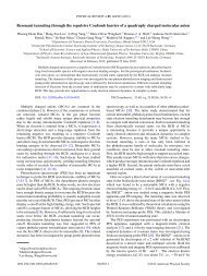
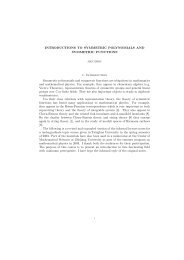
st aat bt cFigure 3: An illustration of transmissions of two signalsbFigure 2: A star-like topology of receiversDefinition 1: S is an acoustic source locating at afixed position in a limited 3D space and can generatean omni-directional sound signal that lasts for a specifiedperiod. For convenience, we also use S to denotethe emitted signal.In Whistle, We assume that the signal S canbe mathematically described in advance. Technically,Whistle does not rely on any specific form of acousticsignals and can be accordingly used for general purposes.In the view of hardware, Whistle involves an acousticsource and several receivers. Receivers are deployedat known locations, serving as the basic infrastructureof a TDOA system. Each receiver has a basic setof hardware, including a speaker, a microphone, andwireless connectors, such as Bluetooth or WiFi. Unlessexplicitly pointing out, the words node and receiverare exchangeable henceforth. Fig. 2 shows a star-likenetwork topology of Whistle. Receivers, in recordingmode, capture sound signals and transmit the timerelatedinformation to an access point. The AP relaysthat information to a laptop for further processing.Using a laptop in Whistle is optional. If we use anode to replace the AP and the laptop, the networkmodel described above is changed into a purely starlikemodel.3. The Design of Whistle3.1. Measuring TDOA by TD2SAs TDOA is important, we describe how to accuratelymeasure it in Whistle. Fig. 4 shows a typical timesequence of two Whistle nodes A and B. Let t A1 andt B1 denote the arriving time of S at the microphonesof A and B, respectively. The TDOA measurement isexactly t B1 − t A1 , if nodes are synchronous. But inWhistle, nodes maintain clocks independently. Evenusing a perfect synchronization scheme, however, westill cannot obtain the exact value of TDOA. Due tothe latency of software and hardware, node A detectsS at t A2 instead of t A1 . The same latency occurs atnode B. Many experimental studies demonstrate thatsuch latencies are inevitable and unpredictable [23].Hence, t A2 − t A1 and t B2 − t B1 are not necessarilythe same (basically different from each other), whichprevents using t B2 −t A2 as the estimate of t B1 −t A1 .To eliminate the uncertainties and errors mentionedabove, we introduce a system sound S ′ to avoid timesynchronization.Definition 2: After receiving the source sound signalS, one of the receivers will emit another soundsignal S ′ , which is called the system sound signal. Thenode emitting S ′ is called base node.With the help of the system sound S ′ , we developa method to measure t B1 −t A1 . As shown in Fig. 4,after a specified time interval τ, node A, as the basenode, emits S ′ from its speaker at time t A3 accordingto its own clock.Theorem 1: For all non-base nodes, they alwaysdetect the system sound signal S ′ after the sourcesound signal S.Proof: LetS be the sound source,athe base node,and b a non-base node. Assume that t a and t b are thepropagation time of S from s to a and from s to b,respectively. In addition, the propagation time of S ′from a to b is denoted by t c . Finally, we use t ab as thetime span lasting from emitting S at s and receivingS ′ at b.The locations of s, a and b construct a triangle inFig. 3, or lie in a straight line. In both cases, wehave t b ≤ t a + t c due to triangle inequality. Sincethe base node encounters a delay between receivingS and emitting S ′ , we have t ab > t a +t c . Therefore,t ab > t b can be obtained, meaning that any non-basenode b always firstly senses S, then S ′ .As shown in Fig. 4, S ′ is emitted from A’s speakerat t A3 , and arrives at the microphones of A and B att A4 and t B3 , respectively. A and B’s CPUs detect S ′at t A5 and t B4 , respectively. According to Theorem 1,t B3 is always later than t B1 . We define the TD2Svalue of one node as the elapsed time between thearrival ofS and the arrival ofS ′ at the node. Obviously,

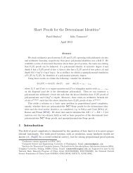
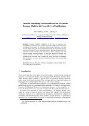
clock at Aclock at BSMICt A1CPUt A2t B1t B2MIC CPUSPEAKERt A3}τS ′MICt A4 t A5t B3MICFigure 4: Time lines of node A and Bt B4T A2S = t A4 −t A1 , T B2S = t B3 −t B1 . The distance ofA’s speaker to B’s microphone (denoted by d AB ) is aconstant since both A and B fix at known locations.In addition, the distance between A’s speaker to itsown microphone (denoted by d AA ) is also a constant.Let T AB denote the TDOA value of A and B, i.e.,T AB = t B1 −t A1 . T AB can be expressed using T A2Sand T B2S , as illustrated in Eq. (1).T AB = t B1 −t A1= (t B3 −t A3 )−(t B3 −t B1 )+(t A3 −t A1 )= (t B3 −t A3 )−(t B3 −t B1 )+(t A4 −t A1 )−(t A4 −t A3 )= d AB−(t B3 −t B1 )+(t A4 −t A1 )− d AAvv= k 1 −T B2S +T A2S −k 2(1)In Eq. (1), k 1 and k 2 are defined as dABvand dAAv ,respectively. Since both k 1 and k 2 are constant, onlyT A2S and T B2S are needed to calculate T AB . The significanceof Eq. (1) is that TDOA can be calculated byTD2S values which can be measured independentlyby asynchronous nodes. The next challenge is how tocalculate the TD2S accurately.3.2. Calculating TD2S AccuratelyIn Fig. 4, since latencies are unpredictable,t A4 −t A1is not necessarily equal to t A5 −t A2 . Therefore, for anode, using two CPU timestamps to calculate a TD2S(traditional synchronization methods often do in thisway) is not promising.Recall that nodes are in the recording state andsamples at a fixed frequency (fHz). In other words,every 1 fsecond, a node senses and translates signalsinto a real or complex number by its A/D converter. Forexample, when the signal S arrives at the microphoneof a node X, X is recording the i-th sample data.After some latency, X’s microphone detects the signalS ′ when its sample counting goes to j (j > iaccording to Theorem 1). Now, we can obtain T X2S ,CorrelationS’1S0−1−2−30 0.5 1 1.5 2 2.5 3 3.5 42 x 104 Sample No.x 10 5Figure 5: One example case of S and S ′the TD2S of nodeX and have T X2S = j−if. Thus, weeliminate the uncertainties that are inherent in the timesynchronization and CPU-timestamp based methods.Basically, a higher sampling rate results in a higheraccuracy. In this paper, the sampling rate is 44.1kHz,which is supported by most COTS devices.3.3. Detecting Sound SignalsAnother critical challenge in Whistle’s design is:how to detect both arrivals of the sound signals S andS ′ ?We assume that both S and S ′ use the same form ofsound signal that is known as a priori. If the signal hasa good auto-correlation property, it is easy and accurateto determine the peak relevant to the arrival of S bycorrelating it with the known signal. Specifically, aftercross-correlation, the two maximal peaks represent thetime-of-arrival of S and S ′ in theory, and the latter oneis S ′ according to Theorem 1 (as shown in Fig. 5).In practice, the highest peak can not always representthe arrival of signal because of multi-path effectsand other uncertainties; we choose the earliest sharppeak in a shadow window of ω 0 points right before themaximal peak instead. We use two parameters: heightand average slope. Average slope is calculated asP = Y peak −Y vallayX peak −X vallay(2)X vallay is the nearest valley point before the peak.Only the peak whose height is larger than Y maxpeak ×TH Y and slope is larger than P maxpeak ×TH P wouldbe chosen. In our implementation, we empirically setω 0 = 5000, TH Y = 0.5, TH P = 0.5.Generally, we can use any signal with good autocorrelationproperty as the reference signal. Consideringthe properties of the built-in speaker and microphoneof a cell phone, in this paper, we select the linearchirp signal (sounds like a whistle) with the frequencychanging from 2kHz to 6kHz as S and S ′ , the durationof the chirp signal is set to 50ms.

3.4. Filtering TD2S OutliersStWe have shown a method using TD2S to calculateTDOA. But sometimes, because of the instability ofsound recording, we get wrong TD2S from defectiverecording which can be attributed to obstacles betweenS and receivers or background noises. Since when andwhere S being emitted are unknown, it is difficult togive a range which the real value of TD2S shouldlocate in. But still we can use a method to tell wrongTD2Ss from the other: majority decision.Suppose that the sound sourceM emitsS at t, whilethe base node N emits S ′ at t ′ . Receivers A and Bboth record the two signals. Thus, the TD2Ss of bothreceivers have the following relation:|∆ TD | = |T A2S −T B2S |= |((t ′ + d ANv )−(t+ d AMv ))−((t ′ + d BNv )−(t+ d BMv ))|= |(d AN −d BN )−(d AM −d BM )|v≤ |d AN −d BN |+|d AM −d BM |v≤ 2d ABv(3)Providing D is the maximum distance among allreceivers in localization (because we have positionsof N i , D can be easily got), for an arbitrary pair ofreceivers, we have |∆ TD | ≤ 2D v. So when we getcorrect TD2Ss of all receivers to form a set D andsort it, we have TD2S max −TD2S min ≤ 2D v .If most of the TD2Ss are correct and a few havesignificant error, elements in D can be divided intothree categories: (1) a majority of elements which arein an interval whose length is shorter than 2D v ; (2) afew elements which are outside of this interval; and(3) the other elements. For arbitrary elements a in (1)and b in (2), |a−b| > 2D v .In this case we can judge category (2) as errorTD2Ss, and only use category (1) to localize S.Obviously, category (1) must have sufficient nodes tocalculate, or we have to use the whole set to get a resultwhich usually has large errors. This kind of divisionbases on the assumption that most of the TD2Ss arecorrect. Such a method works well in practice.Obviously, this method needs redundant nodes.More nodes bring extra localization or measuring cost,but enlarge the set of category (1) and enhance theaccuracy of localization. In fact, there is a trade-offbetween cost and performance. We empirically findt 0t1t 2t 3t 4N 0 t ′ 1 N 1 t ′ 2 N 2 t ′ 3 N 3 t ′ 4 N 4t ′ 0 t ′Figure 6: An illustration of the emissions and receptionsof both source sound signal S and system soundsignal S ′ . N 0 is the base node.that 2 ∼ 3 redundant nodes can increase locationaccuracy significantly.3.5. Framework DesignAfter discussing the details of Whistle, we presentthe Whistle framework design in this section. Asmentioned in Section 2.1, we need M(M ≥ 5) nodesfor 3D localization. Without loss of generality, let N 0be the base node and N i (1 ≤ i ≤ M −1) be a nonbasenode (N 0 is not always the nearest to S). Whistlehas three steps:In step one, nodes start recording, and receive Sby their own microphones. As illustrated in Fig. 6,the signal S is emitted at time t, which will arrive atN 0 , N 1 , . . . , and N M−1 at time t 0 , t 1 ,. . . and t M−1 ,respectively. Note that the time point t or t i (0 ≤ i ≤M−1) in Fig. 6 is regarding to the absolute time line,instead of the time line maintained by any individualnode N i (0 ≤ i ≤ M −1).In step two, the base node N 0 will emit a systemsound signal S ′ at time t ′ (as shown in Fig. 6) after itdetects S. The signal S ′ , of course, will arrive at eachnode after some latency. A node N i (0 ≤ i ≤ M −1)records the time t ′ i of S′ arriving at N i . Every nodemaintains a recording R i which includes both S andS ′ . Correlating R i with the reference signal, using themethod mentioned in Section 3.3, we have t ′ i − t i.For node N i , the TD2S value (t ′ i −t i) depends onlyon N i ’s own clock, provided that the clock of N i isaccurate in a term longer than the period of the soundoccurrence.In the last step, the value of TD2S will be deliveredto a node or an AP for deriving accurate TDOAvalues, based on which the location of the sound sourcecan be finally determined.

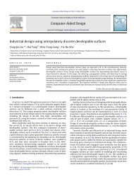
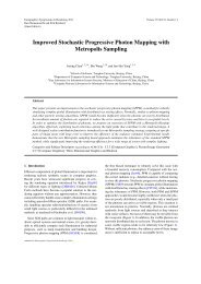
4. Experimental EvaluationyIn this section, we evaluate the performance by a setof experiments on a real testbed.N13604.1. Prototype ConfigurationTo build a prototype, we use eight cell phonesconsisting of six Dopod P800, one O2 XDA Atomand one SonyEricsson XPeria. Each of them has apair of built-in speaker and microphone, and a WiFimodule. We use the O2 cell phone as the base node ,the Sony cell phone as the sound source, and all otherDopod cell phones as receivers. The signals S and S ′are designated to the linear chirp sound.We organize these eight cell phones and an AP(TP-LINK) into a star-like network where all cellphones connect directly to an AP (seen Fig. 2). TheAP relays received data to a laptop(Lenovo T60) forlocation computation. A high performance cell phonecan replace the laptop and AP and serve as a hubconnecting the other cell phones.Using the Windows Mobile 6.0 SDK, we developthe software level of Whistle. For convenience, weimplement a recorder in software level that can enterand quit the recording status periodically and saveautomatically the recorded sound data into a file withthe wav format.4.2. Source of ErrorsWe summarize possible sources of errors in thissection. In Whistle, we get TDOA from TD2S first,and solve the equations according to TDOA. Errorsmay come from both steps. The main factors are asbelow:• Signal to noise ratio (SNR) - Environmentalnoises will always be recorded. If the energy ofthe transmit signals is limited or the frequencyof noises is close to the signals, it is difficult todetect the arrival time of the signals.• Multi-path effects - Because of reflection, anacoustic signal may reach a receiver via differentpaths. Though we take the earliest peak insteadof the highest peak to deal with multipath effects,sometimes the right time point cannot be caught.• Equation solving - Chan’s method performs wellwhen the TDOA measurement errors are small.However, as the errors increase, the performancedegrades. In the experiments, we find that althougha majority of TDOA errors are below0.4ms, a small potion of relatively large errorscontribute a lot to the location error.N6180N5360N0N445N21 2 3 4596 7 810 11 N3 1213 14 15 16Figure 7: Deployment of receivers and acoustic sourcesin 2D case. Unit:cmExcept for some negligible factors, like the propagationspeed variation of sound, there are still otherfactors that may influence localization accuracy. Weplan to use the schemes like [35] to infer hidden failurereasons and detect possible faulty components in thefuture.1354.3. Settings of Test EnvironmentWhistle was evaluated in both 2D and 3D scenarios.In each scenario, according to the error sources mentionedabove, we intentionally conduct the experimentsin three environments:• Case 1-Outdoor, quiet: Whistle is deployed outsidea large gymnasium.• Case 2-Outdoor, noisy: The location is same toCase 1, but loudspeaker plays music nearby.• Case 3-Indoor, quiet: A hall of size about9m×9m×4m.In the following parts, we use “Normal” to denoteCase 1, “Noisy” to Case 2, and “Inside” to Case 3.Through the comparison of three environments, we areexpected to reveal the effect of a single factor (noiseor multi-path effect).We place the sound source at 16 different points ineach environment, and collect 10 repeated samples ofmeasuring data at each point. So totally we have 960different samples under the 2D and 3D deployments.Since temperature may change significantly from startto end, we record temperature once S changes itsposition. The model of sound speed in use is formallydescribed as v air = 331.3+0.6×θ m/s in [1]. Theparameter θ represents the air temperature in Celsius.x

zN1125y#Outlier Location(of 10)54321NoisyInsideNormal00 2 4 6 8 10 12 14 16 18Experimental SequenceN6N343 N0N286 97 1011 14O 12 1516N513N4x#Outlier Location(of 10)54321NoisyInsideNormal00 2 4 6 8 10 12 14 16 18Experimental Sequence(a)The 3D view of the testbedyFigure 9: Outlier number. Figures at top and bottomrepresent the outlier number of 10 samples in 2D and3D cases, respectively.N6N3360N0, N1, N245360N4N5135135xFor 2D or 3D, in all environments, we have thesame deployment of N i and S. Since sound attenuatesrapidly when transmitting in the air, our method isdistance-restricted, so we do our work in an about9m×9m×4m space. We depict 2D deployment inFig. 7 and 3D in Fig. 8, the red points representthe different acoustic source locations and have beenlabeled with different number, the blue points representdifferent receivers. Critical distances are all labeled inthe deployment picture. Our sound source positionsonly occupy 1/4 of the space because it is symmetrical.For simplicity, we use the number associated withthe sound source point as experimental sequence todenote the corresponding test in the following section.4040135N5, N6(b)The top viewzN1N0N250100(c)The right view200360N4, N3Figure 8: Nodes deployment and sound source distributionin 3D experiments. The red points denote differentlocations of S. Unit:cmy4.4. Outlier NumberIn the experiment, we find some results with extremelylarge errors; those errors are from obviouslyfailed experiments which can not get enough eligibleTDOAs. These results significantly lower positionalaccuracy but are of little value and can be easilyseparated from other results. So we identify the resultswith the absolute errors greater than 1m as outlier andexclude them from the results to be used in accuracyevaluation.For example, in a case where a locationS 1 , obtainedby Whistle, is (10,20,30) and the exact sound sourceS = (8,22,30), |x S1 − x S | = 2m > 1m shows thatthe result of S ′ is an outlier.Fig. 9 shows the number of outliers of the 10 samplesin every point of experiments. It is obvious thatthere are only very few outliers in most experiments.The outlier number of inside scene in 3D case isthe largest, but even in this scene, the percentage of

Probability10.80.60.40.2NormalNoisyInside00 0.2 0.4 0.6 0.82D position error(m)mean error of 10 ∼ 20 cm in 3D case and 10 ∼ 21cm in 2D case. They demonstrate that whistle achieveshigh accuracy in all environments.We can see that results in normal environmentsare not always the best. Though noise and multipathincrease the number of outliers, they do not directlyenlarge errors of right results. The consequencesof 3 environments are quite similar. We think thatour system resists multi-path because of the efficientmethod for finding the first peak (seen in Section 3.3),and resists noises because of the good autocorrelationproperty of chirp signal.Probability10.80.60.4NormalNoisyInsideTable 1: 2D critical dataIndicator(cm) Normal Noisy Insidemean error 20.0 20.3 13.750% error 12.7 18.8 10.990% error 38.1 33.7 29.9std 12.8 10.9 12.1outlier percentage 1.25% 5% 0.6%0.200 0.2 0.4 0.6 0.8 13D position error(m)Figure 10: CDF of position errors in 2D and 3D casesoutlier is only 12.5%. The largest outlier number inthe 3D inside scene suggests that WSN localizationin indoor environment is vulnerable due to multipathand obstacles, so researchers often resort to otherequipments in this case. For example, Lionel M. NI etal. [18] propose a location sensing prototype systemnamed LANDMARC that uses RFID for locating objectsinside buildings. The similar idea can be used inour future work to enhance our system’s resistance inindoor environments.In the figure we can see that 2D experiments havemuch less outliers than 3D. We can explain it withthe conclusion which we get from Section 3.4 thatmore redundant nodes bring higher accuracy. The 2Dcase has one more redundant node than 3D, so it iseasier for 2D to avoid outliers. It is observed that bothnoise and multi-path cause more outliers. In 3D casemulti-path gives stronger interference than 2D.4.5. Positional ErrorsFig. 10 depicts the cumulative density function(CDF) of the positional errors in 2D and 3D case. Themean position error and some thresholds can be seenin Tab.1 and Tab.2. The pictures and tables reveal aTable 2: 3D critical dataIndicator(cm) Normal Noisy Insidemean error 14.7 14.4 15.250% error 13.7 13.8 12.890% error 22.8 21.9 28.2std 6.2 7.4 9.9outlier percentage 2.5% 5% 12.5%5. Related WorkMany range-based localization algorithms have beenproposed within a few past decades. Existing workbasically use three types of measurements of acousticsignals: TDOA [24], [19], [32], [9], DOA (directionof arrival) [22], [14], [12], [15] and received signalenergy [25], [26], [4], [21], [3].Cricket [24] is a TDOA based localization system. Ituses concurrent wireless communication and ultrasonicsignal to determine the TDOA value between twonodes referring to their own CPU timestamps. Mahajanet al.’s work [19] uses TDOA measurements to solvea linear equations system similar to ours. Since theirTDOAs are measured by CPU timestamps, clock synchronizationis needed. Moreover, their work is evaluatedonly by simulation. The work in [32] employs 8microphones to obtain the TDOA information, which isfurther used to estimate the bearings of sound sources.Motivated by the applications of monitoring animalsin field, the work in [2], [12] implements andevaluates a sound source localization system calledENSBox [12] and employs it to localize marmot alarmcalls.ENSBox is a DOA-based platform, integrating

an ARM processor, a sensor array, a wireless radioconnector, and precise self-calibration of array positionand orientation.An energy-based localization system is proposed in[4], in which the positions of speakers are estimatedusing an ad hoc microphone array setting and themaximum likelihood estimation method. In [21], aset of methods based on energy measurement aredeveloped, compared, and contrasted. Particularly, aweighted direct least-squares formulation is presented,which incorporates the dependence of unknown parametersleading to high performance.BeepBeep [23] is an acoustic-based ranging systemwith high accuracy. It measures the distance of twocell phones using only their microphones, speakers,and WiFi connection, without leveraging any preplannedinfrastructure. In BeepBeep ranging system,two cell phones emit the same sound signal (Beep)successively, then each phone computes the elapsedtime between the two time-of-arrivals (ETOA). Withthe two ETOAs, the distance between the two phonescan be obtained. Both the two nodes of BeepBeepmust actively participate the ranging process, so thescheme of BeepBeep can be used for TOA localization,but not for TDOA inherently because the to-be-locatedobject (or event) does not necessarily cooperate withreceivers. Whistle extends BeepBeep and develops newtechniques for TDOA localization.Though range-based localization methods can gethigh accuracy, they often need expensive equipmentsand have strict connectivity requirements. Some classicrange-free algorithms like DV-hop [5] and APIT [30]are proposed to implement localization in more extensivecircumstances. DV-hop uses the average distanceof each hop and hop counts to calculate the realdistance between two nodes, so DV-hop has betterperformance in isotropic WSNs. APIT makes tests toknow whether the unknown node is inside the triangleformed by different anchor nodes, and obtains theintersected region of all the triangles that cover theunknown node, then sets the centroid of that regionas the result. APIT has high accuracy but has strictrequirements for connectivity. Mo Li et al. [17] revealthat these range-free schemes fail in anisotropic WSNswith possible holes, and propose the Rendered Path(REP) protocol that is the only protocol for locatingsensors with constant number of seeds in anisotropicWSNs.Several techniques have been proposed for solvingnon-linear TDOA equations. Fang [7] reducedthe computation to the solution of a quadratic or aquartic equation, but his method can not make use ofextra measurements from extra receivers to improveposition accuracy. More general methods with extrareceivers can be found in [10], [28]. They provideclosed-form solutions, but their estimators are not unbiasedand optimum. Abel [13] proposes a divide andconquer (DAC) method which can achieve optimumperformance and unbiased estimator when the datavector is appropriately subdivided, but DAC requiresquiet large Fisher information and is difficult to beimplemented. The Taylor-series method [31], [8] canget high accuracy at reasonable noise levels, but itis computationally intensive because of its iterativecourse and finding a proper initial point to avoidthe convergence problems is not easy. The methodproposed by Chan [33] is noniterative and gives anexplicit solution, and attains the Cramer-Rao lowerbound near the small error region. This method alsohas a higher noise threshold than DAC. In short,the method balances computational complexity andaccuracy, and is accordingly adopted in our work.6. ConclusionIn this paper, we propose an acoustic source localizationframework, Whistle. As a TDOA based system,Whistle changes the scheme of TDOA fundamentally,by releasing the synchronization. In Whistle, severalasynchronous receivers record a target signal and asystem signal. High time resolution is achieved throughtwo-signal sensing and sample counting. Real-worldexperiments are conducted on a testbed system consistingof COTS cell phones. Experiment results show thatWhistle has a mean location error of 10∼20 centimetersin a 9×9×4m 3 3D space. To summarize, Whistleachieves low cost, rapid deployment, and widespreaduse simultaneously.Our ongoing work are: (1) extending Whistle forlarger wireless sensor networks, in which a largenumber of nodes are organized in an ad-hoc manner.There may be quite a lot new problems including errorcontrol and localizability [36] in this multi-hop WSN.Besides, we may have to construct a self-adaptiveWSN topology like [16], for some nodes may run outof energy earlier than the other. Finally, we shouldpay particular attention to the factors that restrict theWSN’s scale and lifetime proposed by Yuan He etal. [34] ; (2) trying to use ordinary sound or voice insteadof a signal that can be mathematically described,and see if we can find some new method for detectingits arrival accurately. (3) using RF signal instead ofacoustic signal. UWB signal is our first choice, as itoffers high time resolution. We will implement Whistleon a UWB localization system and see its effects.

AcknowledgementSpecial thanks to Bo Liu for help in designing thesound recording module and doing the early experiments.This work is supported in part by the NSFChina under Grant No.60803124 and the NationalBasic Research Program of China(973 Program) undergrant No.2006CB303000.References[1] http://en.wikipedia.org/wiki/speed of sound.[2] A. M. Ali, T. C. Collier, and L. Girod. An empericalstudy of collaborative acoustic source localization. InIPSN, pages 41–51, 2007.[3] D. Ampeliotis and K. Berberidis. Linear least squaresbased acoustic source localization utilizing energy measurement.In SAMSP, 2008.[4] M. Chen, Z. Liu, L. He, P. Chou, and Z. Zhang. Energybasedposition estimation of microphones and speakersfor ad hoc microphone arrays. In IEEE Workshop on Applicationsof Signal Processing to Audio and Acoustics,2007.[5] D.Niculescu and B.Nath. Ad hoc positioning system(aps). In IEEE GlobeCom, San Antonio,AZ, November2001.[6] J. Elson, L. Girod, and D. Estrin. Fine-grained networktime synchronization using reference broadcasts. InOSDI, 2002.[7] B. T. Fang. Simple solutions for hyperbolic and relatedposition fixes. IEEE Trans. on Aerospace and ElectronicSystems, 26(5):748–753, September 1990.[8] W. H. Foy. Position-location solutions by taylor-seriesestimation. IEEE Transactions on Aerospace and ElectronicSystems, AES-12(2):187–194, March 1976.[9] K. Frampton. Acoustic self-localization in a distributedsensor network. IEEE Sensor Journal, 6(1):166–172,2006.[10] B. Friedlander. A passive localization algorithm and itsaccuracy analysis. IEEE Journal of Oceanic Engineering,OE-12(1):234–245, January 1987.[11] S. Ganeriwal, R. Kumar, and M. B. Srivastava. Timingsyncprotocol for sensor networks. In SenSys, pages 138–149, 2003.[12] L. Girod, M. Lukac, V. Trifa, and D. Estrin. The designand implementation of a self-calibrating distributedacoustic sensing platform. In SenSys, pages 71–85, 2006.[13] J.S.Abel. A divide and conquer approach to leastsquaresestimation. IEEE Transactions on Aerospace andElectronic Systems, 26(2):423–427, March 1990.[14] K. Kaplan, Q. Le, and P. Molnar. maximum likelihoodmethods for bearings-only target localization. InICASSP, 2001.[15] A. Ledeczi, G. Kiss, B. Feher, P. Volgyesi, andG. Balogh. Acoustic source localization in fusing sparcsedirection of arrival estimates. In ISES, 2006.[16] Mo Li and Yunhao Liu. Underground coal mine monitoringwith wireless sensor networks. ACM Transactionson Sensor Networks (TOSN), 5, March 2009.[17] Mo Li and Yunhao Liu. Rendered path: Rangefreelocalization in anisotropic sensor networks withholes. IEEE/ACM Transactions on Networking (TON),18(1):320–332, February 2010.[18] Lionel M Ni, Yunhao Liu, Yiu Cho Lau and AbhishekPatil. Landmarc: Indoor location sensing using activerfid. ACM Wireless Networks, (WINET), 10:701–710,November 2004.[19] A. Mahajan and M. Walworth. 3-d position sensingusing the differences in the time-of-flights from a wavesource to various receivers. IEEE Trans. on Roboticsand Automation, 17(1):91–95, 2001.[20] M. Maroti, B. Kusy, G. Simon, and A. Ledeczi. Theflooding time synchronization protocol. In SenSys, pages39–49, 2004.[21] C. Meesookho, U. Mitra, and S. Narayanan. On energybasedacoustic source localization for sensor network.IEEE Trans. on Signal Processing, 56(1):365–377, 2008.[22] Y. Oshman and P. Davidson. Optimization of observertrajectories for bearings-only target localization. IEEETrans. on Aerospace and Electronic Systems, 35(3):892–901, 1999.[23] C. Peng, G. Shen, Y. Zhang, Y. Li, and K. Tan.Beepbeep: a high accuracy acoustic ranging system usingcots mobile devices. In SenSys, pages 1–12, Sydney,Australia, November 2007.[24] N. B. Priyantha, A. Chakraborty, and H. Balakrishnan.The cricket location-support system. In Mobicom, pages32–43, 2000.[25] X. Sheng and Y. Hu. Energy based acoustic sourcelocalization. In IPSN, 2003.[26] X. Sheng and Y. Hu. Maximum likelihood multiplesourcelocalization using acoustic energy measurementswith wireless sensor networks. IEEE Trans. on Signaland Processing, 53(1):44–54, 2005.[27] F. Sivrikaya and B. Yener. Time synchronization insensor networks: a survey. IEEE Network, pages 45–50,2004.[28] J. O. Smith and J. S. Abel. The spherical interpolationmethod of source localization. IEEE Journal of OceanicEngineering, OE-12(1):246–252, January 1987.[29] P. Sommer and R. Wattenhofer. Gradient clock synchronizationin wireless sensor networks. In IPSN09: Proceedings of the 2009 International Conferenceon Information Processing in Sensor Networks, pages37–48, Washington, DC, USA, 2009. IEEE ComputerSociety.[30] T. He, C. Huang, B.M. Blum, J.A. Stankovic and T.F.Abdelzaher. Range-free localization schemes for largescale sensor networks. In MOBICOM, pages 81–95,2003.[31] D. J. Torrieri. Statistical theory of passive location systems.IEEE Transactions on Aerospace and ElectronicSystems, AES-20(2):183–198, March 1984.[32] J.-M. Valin, F. Michaud, J. Rouat, and D. Letoumeau.Robust sound source localization using a microphonearray in a mobile robot. In IROS, 2003.[33] Y.T.Chan and K.C.Ho. A simple and efficient estimatorfor hyperbolic location. IEEE Transactions on SignalProcessing, 42(8):1905–1915, August 1994.[34] L. M. Yuan He and Y. Liu. Why are long-term largescalewireless sensor networks difficult: early experiencewith greenorbs. Mobile Computing and CommunicationsReview, 14(2):10–12, 2010.[35] K. L. Yunhao Liu and M. Li. Passive diagnosis forwireless sensor networks. IEEE/ACM Transactions onNetworking (TON), 18(4):1132–1144, August 2010.[36] X. W. Yunhao Liu, Zheng Yang and L. Jian. Location,localization, and localizability. Journal of ComputerScience and Technology, 25(2):274–297, March 2010.