Industrial design using interpolatory discrete developable surfaces

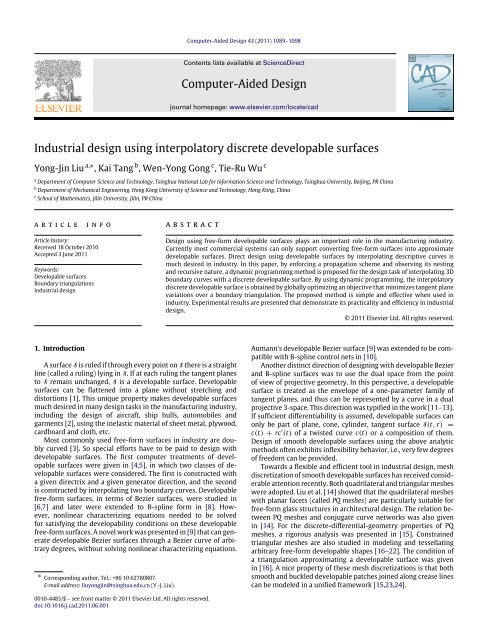
Computer-Aided Design 43 (2011) 1089–1098Contents lists available at ScienceDirectComputer-Aided Designjournal homepage: www.elsevier.com/locate/cadIndustrial design using interpolatory discrete developable surfacesYong-Jin Liu a,∗ , Kai Tang b , Wen-Yong Gong c , Tie-Ru Wu ca Department of Computer Science and Technology, Tsinghua National Lab for Information Science and Technology, Tsinghua University, Beijing, PR Chinab Department of Mechanical Engineering, Hong Kong University of Science and Technology, Hong Kong, Chinac School of Mathematics, Jilin University, Jilin, PR Chinaa r t i c l ei n f oa b s t r a c tArticle history:Received 18 October 2010Accepted 3 June 2011Keywords:Developable surfacesBoundary triangulationsIndustrial designDesign using free-form developable surfaces plays an important role in the manufacturing industry.Currently most commercial systems can only support converting free-form surfaces into approximatedevelopable surfaces. Direct design using developable surfaces by interpolating descriptive curves ismuch desired in industry. In this paper, by enforcing a propagation scheme and observing its nestingand recursive nature, a dynamic programming method is proposed for the design task of interpolating 3Dboundary curves with a discrete developable surface. By using dynamic programming, the interpolatorydiscrete developable surface is obtained by globally optimizing an objective that minimizes tangent planevariations over a boundary triangulation. The proposed method is simple and effective when used inindustry. Experimental results are presented that demonstrate its practicality and efficiency in industrialdesign.© 2011 Elsevier Ltd. All rights reserved.1. IntroductionA surface S is ruled if through every point on S there is a straightline (called a ruling) lying in S. If at each ruling the tangent planesto S remain unchanged, S is a developable surface. Developablesurfaces can be flattened into a plane without stretching anddistortions [1]. This unique property makes developable surfacesmuch desired in many design tasks in the manufacturing industry,including the design of aircraft, ship hulls, automobiles andgarments [2], using the inelastic material of sheet metal, plywood,cardboard and cloth, etc.Most commonly used free-form surfaces in industry are doublycurved [3]. So special efforts have to be paid to design withdevelopable surfaces. The first computer treatments of developablesurfaces were given in [4,5], in which two classes of developablesurfaces were considered. The first is constructed witha given directrix and a given generator direction, and the secondis constructed by interpolating two boundary curves. Developablefree-form surfaces, in terms of Bezier surfaces, were studied in[6,7] and later were extended to B-spline form in [8]. However,nonlinear characterizing equations needed to be solvedfor satisfying the developability conditions on these developablefree-form surfaces. A novel work was presented in [9] that can generatedevelopable Bezier surfaces through a Bezier curve of arbitrarydegrees, without solving nonlinear characterizing equations.∗ Corresponding author. Tel.: +86 10 62780807.E-mail address: liuyongjin@tsinghua.edu.cn (Y.-J. Liu).Aumann’s developable Bezier surface [9] was extended to be compatiblewith B-spline control nets in [10].Another distinct direction of designing with developable Bezierand B-spline surfaces was to use the dual space from the pointof view of projective geometry. In this perspective, a developablesurface is treated as the envelope of a one-parameter family oftangent planes, and thus can be represented by a curve in a dualprojective 3-space. This direction was typified in the work [11–13].If sufficient differentiability is assumed, developable surfaces canonly be part of plane, cone, cylinder, tangent surface S(t, r) =c(t) + rc ′ (t) of a twisted curve c(t) or a composition of them.Design of smooth developable surfaces using the above analyticmethods often exhibits inflexibility behavior, i.e., very few degreesof freedom can be provided.Towards a flexible and efficient tool in industrial design, meshdiscretization of smooth developable surfaces has received considerableattention recently. Both quadrilateral and triangular mesheswere adopted. Liu et al. [14] showed that the quadrilateral mesheswith planar facets (called PQ meshes) are particularly suitable forfree-form glass structures in architectural design. The relation betweenPQ meshes and conjugate curve networks was also givenin [14]. For the discrete-differential-geometry properties of PQmeshes, a rigorous analysis was presented in [15]. Constrainedtriangular meshes are also studied in modeling and tessellatingarbitrary free-form developable shapes [16–22]. The condition ofa triangulation approximating a developable surface was givenin [16]. A nice property of these mesh discretizations is that bothsmooth and buckled developable patches joined along crease linescan be modeled in a unified framework [15,23,24].0010-4485/$ – see front matter © 2011 Elsevier Ltd. All rights reserved.doi:10.1016/j.cad.2011.06.001

Y.-J. Liu et al. / Computer-Aided Design 43 (2011) 1089–1098 1091Fig. 1.The interface of the working system. Left: A screen snapshot. Right: A typical working environment of the sketching system.Table 1Some notations used in this paper.NotationT(P)OT(P)πP 2DSupporting line segment (SLS)A rung ⟨m, n⟩A gate rungA regular rungOptimal rungBridge triangulation BT(P)OBT(P)L(i)MeaningA boundary triangulation of PThe optimal boundary triangulation of PThat maximizes the measure M(T).The sketch planeThe projection of P onto πA line segment inside P that starts at someVertex p i ∈ P, goes through some concaveVertex p j ∈ P and ends in an edge of P.A line segment connecting p m and p n that isEntirely inside P except its two ends.A rung that is a part of an SLSA rung that is not a gate rungA rung that is an edge in OT(P)A boundary triangulation in which everytriangle has at most two rungs.The optimal bridge triangulation of P thatMaximizes the measure M(BT).The set of valid rungs emanating from p iFig. 2. Polyline resampling: Supporting line segment (SLS), gate and regular rungs.Let P discretize smooth curves C. The vertices in P are orientedso that when one walks along the P, the interior region boundedby P (P possibly has several disjoint closed polylines) is always onthe right-hand side. For any boundary triangulation T of P, eachedge e ∈ T consists of two vertices p i , p j ∈ V P . Denote the tangentvectors in the smooth curves C at the positions of p i , p j by t i , t j ,respectively. The discrete normal vector to the discrete surface Tat position p i , with respect to p j , is defined by n j i= (p j−p i )×t i∥(p j −p i )×t i ∥ . Atwist measure of edge e = (p i , p j ) is defined bym(e) =n j · i ni − 1, j e ∉ P0 e ∈ P.The discrete developability of T is measured by the total twistM(T):M(T) =m(e). (1)e∈T,e∉PSince the measure m(e) is always less than or equal to zero,and m(e) = 0 only if perfect developability is achieved, givenan T , the larger M(T) is, the better the developability obtained.Note that a similar measure of developability for semi-discretesurfaces is used in [31] to define developable surface strips.Among all the possible boundary triangulations of P, let OTbe the triangulation that maximizes the measure M(T). If thesampling density of P is increased to the infinate, the boundarytriangulation OT(P) maximizing the developablity measure (1)converges to a smooth developable surface or a composition ofseveral developable surfaces joined along crease lines, while otherboundary triangulations may converge only to a ruled surface. Inthis paper, OT(P) is regarded as a quasi-developable surface of P.Fig. 3. Polyline P partitioning by a rung l: Two halves P(l + ) and P(l − ), and twobridge triangles from l in P(l + ).4.1. Optimal bridge triangulation of a single closed curveLet π be the sketch plane specified in Section 3. Denote theprojection of P onto π by P 2D . Let P 2D be indexed using the righthand-siderule specified at the beginning of Section 4. With thisorder, we make no distinction between sampling P and its polyline.A point in P is said to be concave in R 2 if its interior angle is largerthan π, otherwise it is convex in R 2 . Refer to Fig. 2. A supportingline segment (SLS) of P is a line segment inside P that starts at somevertex p i ∈ P, supports (goes through) some concave vertex p j ∈ Pand ends in an edge of P. Assume that the original polyline P can beresampled so that for any SLS, both its ends are vertices in P. A linesegment connecting p m and p n , denoted as ⟨m, n⟩, is called a rungif it is entirely inside P except its two ends. In particular, it is calleda gate rung if it is a part of an SLS, e.g., ⟨i, j⟩ in Fig. 2; otherwise, itis a regular rung. When a rung ⟨i, j⟩ is referred to, it is assumed thati < j.As P is simple, any rung l = ⟨i, j⟩ divides P into two halves.Denote by P(l + ) = P(⟨i, j⟩ + ) the half that has the vertex p i+1 andby P(l − ) = P(⟨i, j⟩ − ) the other half (Fig. 3). If a rung l is an edge

1092 Y.-J. Liu et al. / Computer-Aided Design 43 (2011) 1089–1098Fig. 4. Topological structure of P around a gate rung ⟨i, j⟩.Fig. 5. Change of topological structure when a gate rung is encountered.in an OT of P (referred to as an optimal rung), it is obvious that thefollowing equations hold:M(OT(P)) = M(OT(P(l + ))) + M(OT(P(l − ))) + m(l). (2)Recall that OT(P) is the optimal triangulation of sampling P underthe twist measure M(·). We first study a particular type of triangulationcalled bridge triangulation (BT): BT is a boundary triangulationin which every triangle has at most two rungs.Refer to Fig. 3. For any optimal bridge triangulation (OBT) ofP(l + ), it must have either rung ⟨i, j − 1⟩ or ⟨i + 1, j⟩ as an edge. Thefollowing recursive rule holds for a regular optimal rung l = ⟨i, j⟩:M(OBT(P(⟨i, j⟩ + )))= max{M(OBT(P(⟨i + 1, j⟩ + ))) + m(⟨i + 1, j⟩),M(OBT(P(⟨i, j − 1⟩ + ))) + m(⟨i, j − 1⟩)} (3)with the boundary condition that this recursion terminates at j =(i + 2) mod n. The recursive rule for M(OBT(P(⟨i, j⟩ − ))) is definedsimilarly. Given rule (3), the dynamic programming method [32]can be applied to find an OBT of P if the projection of P onto thesketch plane is convex.The dynamic programming method has been used in [18,22]to obtain an optimal bridge triangulation of a rectangular strip.However, concave vertices are not considered in [18,22]. In general,the projection of P could enclose a concave region in the sketchplane π. Refer to Fig. 4. Consider a gate rung l = ⟨i, j⟩ with jbeing the supported concave vertex and k the vertex on the otherend of the associated SLS. At a concave vertex p j , P(⟨i + 1, j⟩ + ) iswell defined, but not P(⟨i, j − 1⟩ + ) since ⟨i, j − 1⟩ is not a rung (itintersects P). To extend rule (3) for including concave vertices, thefollowing recursive rule is established for a gate rung ⟨i, j⟩:M(OBT(P(⟨i, j⟩ + )))= max{M(OBT(P(⟨i + 1, j⟩ + ))) + m(⟨i + 1, j⟩),M(OBT(P(⟨i, k − 1⟩ + ))) + m(⟨i, k − 1⟩)+ M(OBT(P(⟨k − 1, j⟩ + ))) + m(⟨k − 1, j⟩)}. (4)In rule (4), we assume i < k < j after a cyclic reordering of P.Rule (4) considers the case that the gate rung ⟨i, j⟩ is moving out ofa pocket. The opposite case is that the rung propagation enters apocket, as shown in Fig. 5. The corresponding rule of this oppositecase is as follows:M(OBT(P(⟨i, j⟩ + ))) = M(OBT(P(⟨i, k⟩ + ))) + m(⟨i, k⟩)+ M(OBT(P(⟨k, j⟩ + ))) + m(⟨k, j⟩). (5)Generally in each SLS there is only one concave vertex. Inrare scenarios, degenerate cases may occur that several concavevertices lie in an SLS. Refer to Fig. 6: Two concave vertices p j andp k lie in an SLS. In this case, we duplicate p k with a dummy convexvertex p ′ k . Then we treat (i, j, k′ ) and (i, k, l) as two different SLSs.Applying dynamic programming on this treatment will producea dummy triangle △(i, k, k ′ ) in an optimal triangulation OT . Toprocess degeneracies, we find and delete all the dummy trianglesin OT . Our split-dummy-vertex method falls into the symbolicperturbation strategy in [33] in which elegant analysis on thisstrategy is discussed in a much broader scope.Given rules (2–5), the standard top–down dynamic-programmingalgorithm [32] is applied to find an OBT of P. To start upthe algorithm, consider an arbitrary convex vertex p i . Let L(i) bethe set of valid rungs emanating from p i . Any valid triangulationof P must contain either a rung in L(i) or the rung ⟨i − 1, i + 1⟩.Therefore by applying rule (2) to every rung in L(i)∪{⟨i−1, i+1⟩},the triangulation with the maximum twist measure (1) is an OBTof P.A memorization technique [32] is used to improve the efficiencyof the dynamic programming method while maintaining thetop–down strategy. Explicitly, two n × n scalar matrices M + andM − are utilized to record the twist values M(OBT(P⟨i, j⟩ + )) andM(OBT(P⟨i, j⟩ − )). i.e., M + [i, j] = M(OBT(P⟨i, j⟩ + )) and M − [i, j] =M(OBT(P⟨i, j⟩ − )). In addition to obtain the maximum twist valueof the OBT, another n × n structural matrix N is built to record thelocal advancement of the rungs returned from rules (2–5), so thatthe final OBT can be reconstructed. The total running time of thememorized dynamic-programming algorithm is O(n 3 ), where n isthe number of sample points in P.4.2. Optimal triangulation of a single closed curveThe optimal triangulation obtained by applying the rules (2–5)is limited to bridge triangulation only, i.e., every triangle must havean edge in P. Thus the shape shown in Fig. 7 cannot be found. Nextwe develop a recursive rule for the general optimal triangulationOT .Let l = ⟨i, j⟩ be a rung, either regular or gate. A vertex p k is saidto be rung-visible from l if both ⟨i, k⟩ and ⟨k, j⟩ are rungs (again weassume i < k < j after a cyclic reordering). Since P is simple, if p kis rung-visible, the triangle (p i , p j , p k ) lies entirely inside P exceptthe three vertices. Denote by V(i) the set of indices of the verticesrung-visible from p i , the following rule for the general optimaltriangulation is established:M(OT(P(⟨i, j⟩ + ))) = max{M(OT(P(⟨i, x⟩ + ))) + m(⟨i, x⟩)+ M(OT(P(⟨x, j⟩ + )))+ m(⟨x, j⟩) : x ∈ V(i) ∩ V(j) ∩ P(⟨i, j⟩ + )}.,Fig. 6. Handling degenerate cases when multiple concave vertices lie in a SLS.

Y.-J. Liu et al. / Computer-Aided Design 43 (2011) 1089–1098 1093and then convert P into a simple polygon P ′ , for which the rules(2–6) can be applied.To guarantee OT(P) = OT(P ′ ), the choice of cutting rungs isimportant. Let v i c be a vertex on the convex hull of a hole H i. v i c iscalled a sink if every rung in L(v c ) connects H i to Q . We have thefollowing two properties:Fig. 7. A composite developable surface: Three cone patches joined with a plane,and the boundary curve is shown in red. (For interpretation of the references tocolour in this figure legend, the reader is referred to the web version of this article.)Recall that if e ∈ P, m(e) = 0, i.e., M(T) does not count theedges in P, we can slightly modify the above rule to include theOBT case:M(OT(P(⟨i, j⟩ + ))) = max{M(OT(P(⟨i, x⟩ + ))) + m(⟨i, x⟩)+ M(OT(P(⟨x, j⟩ + )))+ m(⟨x, j⟩) : x ∈ (V(i) ∪ i + 1)∩(V(j) ∪ j − 1) ∩ P(⟨i, j⟩ + )}. (6)By using rules (2) and (6) with the boundary conditions specifiedby rules (2–5), the general OT is found after the recursion of thetop–down dynamic-programming algorithm. Note that the rungvisibilityis locally updated after each marching step, so that V(i)and V(j) only contain non-visited vertices.To implement the algorithm, we need to compute the rungvisibilityset V(i) for all vertices in P. This equals building a visibilitygraph VG(P) of a simple polygon P and removing the edges in Pfrom VG(P). We use the optimal output-sensitive algorithm in [34]to build VG(P) in O(m + n log log n) time, where m is the numberof edges in VG(P).4.3. Optimal triangulation of multiple closed curvesGenerally a developable surface can have multiple closed curvesas its boundary. Our sketching interface provides an flexibletool for constructing this kind of boundary with continuousinteractive editing: First, multiple planar closed curves that enclosea multiple-connected region are specified in the sketch plane; thenthe handle points of B-spline curves are modified along the normaldirection to make 3D boundaries.Consider a non-simple polygon P in the sketch plane which isbounded by the curve set Ω = {Q , H 1 , H 2 , . . . , H m }, where Q isthe external closed boundary curve and H 1 , H 2 , . . . , H m are m nonintersectingholes forming the internal boundary of P. The verticeson holes are ordered counter-clockwise, so that when one walksalong the boundary Ω, the interior region is always on the righthandside. Refer to Fig. 8. Our strategy is to cut P along some rungsProperty 4.1. If three sequential vertices v i j−1 , vi j , vi j+1 of H i lie on theconvex hull of H i , then any boundary triangulation of P must containat least one rung in L(v i j ) that connects H i to another boundary curvein Ω \ H i .Proof. Denote the three sequential vertices of H i that lie on theconvex hull of H i , in counter-clockwise order, by v i j−1 , vi j and vi j+1 .If Property 4.1 does not hold, then all the rungs in L(v i) j connect vi jto some other vertex v i k of H i. Since (1) any boundary triangulationT of P contains v i jas a vertex which has a degree no smaller than3, and (2) two edges (v i , j−1 vi) j and vi, j vi j+1lie on the convex hull ofH i , all remaining edges (a nonempty set) in T which are incident tov i j must cross the interior of hole H i. That is a contradiction to thedefinition of boundary triangulation. So Property 4.1 holds. □Property 4.2. If three sequential vertices v i j−1 , vi j , vi j+1 of H i lie on theconvex hull of {H 1 , H 2 , . . . , H m }, then v i jis a sink and any boundarytriangulation of P must contain at least one rung in L(v i j) that connectsH i to Q .Proof. Let Ω be the convex hull of inner boundaries (H 1 , H 2 , . . . ,H m ), and v i j−1 , vi j , vi j+1 be three sequential vertices of H i, in counterclockwiseorder, lying on Ω. If v i jis not a sink, then all the rungs inL(v i) j connect vi jto some other vertex v j k of H j. Since v i , j−1 vi j , vi j+1lies on Ω, all the rungs in L(v i) j must cross the interior of hole H i, acontradiction. So Property 4.2 holds. □Since boundary Ω consists of smooth curves, if the sampling ofΩ is sufficiently dense, a sink vertex always exists. Based on theProperties 4.1 and 4.2, we use the following procedure to find anoptimal set of cutting rungs.Step 1. Let external boundary be Q and internal boundary H ={H 1 , H 2 , . . . , H m }.Step 2. Find the convex hull of H and identify a sink vertex v c .Step 3. For every rung l in L(v c ).Step 3.1. Cut the region using l which connects a H k to Q ;Step 3.2. Set Q = Q ∪ H k and H = H \ H k ;Step 3.3. If H ≠ ∅.Step 3.3.1. Go to Step 2.Step 3.4. Else stop.The convex hull of a simple polygon can be efficiently foundin linear time [35]. To find the convex hull of several polygons,we apply the marriage-before-conquest method in [36] that runsin O(n log h) time, where n is the number of vertices of inputpolygons and h is the number of vertices on the output hull. Finally,for helping identify sink vertices, we use the output-sensitivescheme in [37] to build the visibility graph of simple polygon Q,Fig. 8. Cutting a non-simple polygon into a simple one along some rungs.

1094 Y.-J. Liu et al. / Computer-Aided Design 43 (2011) 1089–1098a b c(a) Sample a multi-connectedregion on a conic surface(b) The optimal triangulationof our method(c) The optimal ruled surfacein [22]Fig. 9. Reconstruction of a multi-connected region in a conic section, using the proposed optimal triangulation method and the optimal ruled surface method [22],respectively. Dash circles outline the major difference in triangulations. The developability is visualized using Gaussian images.Top viewBottom view(a) Optimal triangulation of acomposite boundary(b) Bridge triangulation of thesame boundary in (a)(c) Two triangulations arealigned together alongthe same boundaryFig. 10. Developable surface reconstruction by interpolating a composite boundary: (a) the optimal triangulation; (b) the optimal bridge triangulation; (c) two triangulationshave the exact same boundary.with respect to m polygonal obstacles {H 1 , H 2 , . . . , H m }, in optimalO(E + T + m log n) time, where E is the size of the visibilitygraph and T is the time required to triangulate the simple polygonwith obstacles. The overall dynamic-programming algorithm formultiple close curves has the time complexity of O(n m+3 ) in theworst case. Since we use several output-sensitive schemes in thealgorithm, in all our experiments, our algorithm is fast: If thereare a few hundred sample points, the running time is less thanone second. In our experiments, all the tests are performed on aCore2Duo 2.4 GHz laptop computer with 2GB of memory.5. ExperimentsThe proposed discrete developable surface design system(Fig. 1) is built on the platform of Visual C++.net with Qt 4 GUI.The distinct features of the system include supporting sketch inputand supporting free-form shape design using discrete developablesurfaces. Below we present a series of experiments to demonstratethese features. Since along each ruling of a developable surface S,the tangent plane does not change, the Gaussian image of S is aspherical arc. Based on this property, we use the Gaussian imageto visualize the quality of discrete developability.Developable surface design with a multi-connected region. As asimple and demonstrative example, we sample a multi-connectedregion on a (developable) conic surface (Fig. 9(a)). Given thesampled boundary P, we apply our algorithm to reconstruct thedevelopable patch interpolating P (Fig. 9(b)). Fig. 9(c) shows thecomparison to the optimal ruled surface using the method in [22].Since our algorithm minimizes the tangent plane variation and

Y.-J. Liu et al. / Computer-Aided Design 43 (2011) 1089–1098 1095Table 2Statistic data of the models presented in Section 5. The interactive design time includes the creative idea generation.Model name Pieces of dev. patches Triangle number Interactive design time (min)Tent (Fig. 12 bottom) 4 407 15Lantern (Fig. 13) 12 1152 5Flower (Fig. 14) 36 2304 75Ship hull (Fig. 15) 4 160 20Car hood (Fig. 16) 8 5928 60Architectural base (Fig. 17 bottom) 1 264 10Fig. 11. Quadrilateral meshes converted from the optimal triangulations shown inFigs. 9(b) and 10(a), respectively.the optimal triangulation is not limited to bridge triangles, it isclearly shown in the companion Gaussian images that our optimaltriangulation of P better approximates the developable surfacethan the optimal ruled surface method in [22]. Other examplesof free-form surface design with a multi-connected region arepresented in Figs. 12 and 17. Compared to the previous work[18,20,22] that builds bridge triangulations in rectangular strips,the shape that encloses multiple inner holes in the sketch plane π(e.g., the ones shown in Figs. 12 and 17) can only be modeled bythe method proposed in this paper.Composite developable surface design. Our algorithm designsdevelopable surfaces by interpolating given boundaries. In thismanner composite developable surfaces can be efficiently builtas follows. Given two pieces of patch boundaries with consecutiveportions P 1 = {b 1, . . . , 1 bn} 1 and P 2 = {b 1, . . . , 2 bm 2}, if someportions in two patches satisfy b i = 1bj 2, then the two patchescan be joined together and we denote this by P 1 ⊕ P 2 ={. . . , b i−11, b j+12, . . . , b j−12, b i+11, . . .}. We can further impose continuityconditions such as G 1 or G 2 between boundary segmentsb i−11, b j+12and b j−12, b i+11, so that smooth composite boundary P 1 ⊕P 2 can be achieved. Fig. 10 shows developable surfaces interpolatingsmoothly joined composite boundary P which is akin to thecomposite example shown in Fig. 7. Fig. 10(a) shows the optimaltriangulation OT(P) and Fig. 10(b) shows the special bridge optimaltriangulation OBT(P) from [22]. The reconstruction qualityof these two triangulations is shown in the Gaussian images. Thisexample clearly demonstrates that using only bridge triangles canfind limited success in a few special cases [20,22] while the proposedoptimal triangulation is a generalization suitable in a widerrange of applications.Connection to quadrilateral meshes. Both quadrilateral and triangularmeshes are widely used for a discrete surface representationin industry. An optimal triangulation obtained from theproposed algorithm can be post-processed into a quadrilateralmesh, which in turn can serve as an initial input towards an optimalPQ mesh [14,15]. Let the optimal triangulation OT(P) of boundaryP be denoted by a graph G(V, E), where V ⊆ P. For each vertexv ∈ V , if the degree of vertex deg(v) > 3, then v is called a candidatevertex. For each edge e ∈ E, if both its vertices are candidatevertices, then e is called a candidate edge. For each candidateedge ce, denote the dihedral angle of two triangles incident to ce byDih(ce). The following algorithm converts an optimal triangulationOT(P) = G(V, E) into a quadrilateral mesh.1. Compute the degrees of all vertices in G and identify all thecandidate vertices.2. Identify all the candidate edges and put them into a heap Hindexed by Dih(ce).3. While H is not empty3.1. Extract a candidate edge ce with minimum index from H.3.2. Delete ce from E and locally update H.4. Update G and identify all the candidate vertices in G.5. For each candidate vertex vFig. 12. Two tent models. Top: Composite quasi-developable surface design without holes. Bottom: Windows are modeled by trimming two patches with inner holes.

1096 Y.-J. Liu et al. / Computer-Aided Design 43 (2011) 1089–1098Fig. 13. A Chinese lantern model made up of 12 quasi-developable patches with 1152 triangles.Fig. 14. A flower model made up of 9 petals with 2304 triangles: (a) the rendering; (b) one petal; (c) the planar flattening of (b).Fig. 15. A ship hull model. Top row: The ship hull model in Gouraud shadingand wireframe representations. Bottom row: a papercraft model made from planarflattening of discrete developable patches.5.1. Duplicate the vertex with deg(v) − 2 copies and distributethe copies in a predefined small interval (−ε, ε) centeredat position of v on P.Fig. 16. A car hood model made up of 8 quasi-developable patches.5.2. Locally update the connectivity of v in the subgraphincident to v, such that each copy of v has degree 3.

Y.-J. Liu et al. / Computer-Aided Design 43 (2011) 1089–1098 1097Fig. 17. Architectural base design with a projected multi-connected region. Left: One inner hole. Right: Two inner holes.Fig. 11 shows two examples of quadrilateral meshes convertedfrom the examples shown in Figs. 9(b) and 10(a). As shown inFig. 11, few planar polygons other than quadrangles may be outputfrom the above algorithm and they can be further converted intoquadrilaterals using the methods in [38].Evaluation of sketch-based interface. To the authors’ best knowledge,there is no commercial system that offers the function ofdesign directly using free-form developable surfaces. In [18] aplug-in module of approximating free-form B-spline surface by developablestrips with a controllable global error bound is developedin the CATIA V5 R16 system. We present both the CATIA V5R16 system with the developable approximation module and theproposed sketching system to nine college students (4 females and5 males) aged between 17 ad 23. The same design task to be fulfilledby both systems was assigned to the nine users. Then weasked the users to comment on both systems. All the users commentedthat CATIA is powerful, but it is not easy to learn at firstglance. All the users also commented that the sketching system issimple and easy to use, and the design intent of users can be addressedfluently. Table 2 summarizes the interactive design time(including the creative idea generation) of six sophisticated modelsusing the sketching interface. With this data, we conclude thatthe sketching interface explores a point in the tradeoff betweenexpressiveness and naturalness, with which users can focus onthe task without excessively switching among menus, buttons andkeyboard hits.Aesthetic and industrial design. The sketching system providesa promising tool for using developable surfaces in aesthetic andindustrial design. Figs. 12 and 13 show two tents and a Chineselantern, which are made of 4 and 12 quasi-developable patches,respectively. Fig. 14 shows a composite flower model that uses36 quasi-developable patches: One graduate student took 75 minto sketch all the boundaries and a total of 2304 triangles aregenerated by the optimal triangulations. A ship hull consistingof 4 quasi-developable patches, in a symmetric configuration, isshown in Fig. 15 in which the papercraft model constructed fromplanar development is also presented. A sophisticated car modelis presented in Fig. 16 in which the hood is designed using acomposite quasi-developable surface. An example in architecturaldesign is presented in Fig. 17. Table 2 summarizes the statisticsdata of all the models (developable patches, number of triangles,and the interactive design time using the sketching interface). Oncethe boundary curves are specified, the models in all the examplesare generated in time between one to one hundred milliseconds, ona Core2Duo 2.4 GHz laptop computer with 2GB memory, indicatingthat real-time shape manipulation and modification are achievedby the proposed system.6. ConclusionsIn this paper, we have presented a dynamic programmingmethod for generating optimal discrete developable surfacesinterpolating given 3D boundary curves. Compared to previousworks, a distinct feature of the proposed method is that ourdesign system separates developable surface modeling into threephases: (1) interactive design of boundary curves in a sketchingplane, (2) interactive modification along normal directions, and(3) automatic generation of discrete developable surfaces thatinterpolate the given boundaries. Unlike previous strip-basedmethods, on the sketching plane, the boundaries in our systemcan enclose several inner holes and then form a multi-connectregion. To facilitate the proposed system, a sketching interfaceis utilized that offers a design tool to allow designers toconstruct sophisticated free-form shapes naturally and efficiently.Experimental results are presented, showing that sophisticatedfree-form developable surfaces can be designed by users in a lowcognitive load, by using the three-phase design system with asketching interface.AcknowledgmentsThe authors thank the reviewers for their comments that helpimprove this paper. This work was supported by the NationalScience Foundation of China (Project 60970099, 60736019),the National Basic Research Program of China 2011CB302202and Tsinghua University Initiative Scientific Research Program20101081863.References[1] do Carmo M. Differential geometry of curves and surfaces. Prentice-Hall, Inc.;1976.[2] Liu Y, Zhang D, Yuen M. A survey on CAD methods in garment design.Computers in Industry 2010;61(6):576–93.[3] Farin G. Curves and surfaces for CAGD. 5th ed. Morgan Kaufmann Pub.; 2002.[4] Gurunathan B, Dhande S. Algorithms for development of certain classes ofruled surfaces. Computers & Graphics 1987;11(2):105–12.[5] Weiss G, Furtner P. Computer-aided treatment of developable surfaces.Computers & Graphics 1988;12(1):39–51.[6] Aumann G. Interpolation with developable Bezier patches. Computer AidedGeometric Design 1991;8(5):409–20.[7] Lang J, Roschel O. Developable (1, n)-Bezier surfaces. Computer AidedGeometric Design 1992;9(4):291–8.[8] Maekawa T, Chalfant J. Design and tessellation of b-spline developablesurfaces. Transactions of the ASME. Journal of Mechanical Design 1998;120(3):453–61.[9] Aumann G. A simple algorithm for designing developable Bezier surfaces.Computer Aided Geometric Design 2003;20(8–9):601–19.

1098 Y.-J. Liu et al. / Computer-Aided Design 43 (2011) 1089–1098[10] Fernandez-Jambrina L. B-spline control nets for developable surfaces.Computer Aided Geometric Design 2007;24(4):189–99.[11] Bodduluri R, Ravani B. Design of developable surfaces using dualitybetween plane and point geometries. Computer-Aided Design 1993;25(10):621–32.[12] Bodduluri R, Ravani B. Geometric design and fabrication of developable Bezierand b-spline surfaces. Transactions of the ASME. Journal of Mechanical Design1994;116(4):1042–8.[13] Pottmann H, Farin G. Developable rational Bezier and b-spline surfaces.Computer Aided Geometric Design 1995;12(5):513–31.[14] Liu Y, Pottman H, Wallner J, Yang Y, Wang W. Geometric modeling with conicalmeshes and developable surfaces. In: ACM SIGGRAPH 2006. 2006. p. 681–9.[15] Kilian M, Flory S, Chen Z, Mitra N, Sheffer A, Pottmann H. Curved folding. In:ACM SIGGRAPH 2008. 2008. p. Article No. 75.[16] Frey W. Boundary triangulations approximating developable surfaces thatinterpolate a closed space curve. International Journal of Foundations ofComputer Science 2002;13(2):285–302.[17] Julius D, Kraevoy V, Sheffer A. D-charts: quasi-developable mesh segmentation.In: Eurographics 2005. 2005. p. 581–90.[18] Liu Y, Lai Y, Hu S. Stripification of free-form surfaces with global error boundsfor developable approximation. IEEE Transactions on Automation Science andEngineering 2009;6(4):700–9.[19] Rose K, Sheffer A, Wither J, Cani M, Thibert B. Developable surfaces fromarbitrary sketched boundaries. In: Eurographics symposium on geometryprocessing. 2007. p. 163–72.[20] Tang K, Wang C. Modeling developable folds on a strip. Journal of Computingand Information Science in Engineering 2005;5(1):35–47.[21] Wang C. Computing length-preserved free boundary for quasi-developablemesh segmentation. IEEE Transactions on Visualization and ComputerGraphics 2008;14(1):25–36.[22] Wang C, Tang K. Optimal boundary triangulations of an interpolating ruledsurface. Journal of Computing and Information Science in Engineering 2005;5(4):291–301.[23] Frey W. Modeling buckled developable surfaces by triangulation. Computer-Aided Design 2004;36(4):299–313.[24] Liu Y, Tang K, Joneja A. Modeling dynamic developable meshes by the Hamiltonprinciple. Computer-Aided Design 2007;39(9):719–31.[25] Bo P, Wang W. Geodesic-controlled developable surfaces for modeling paperbending. In: Eurographics 2007. 2007. p. 365–74.[26] LaViola J. Sketch-based interfaces: techniques and applications. In: ACMSIGGRAPH. Course notes 3. 2007.[27] Ma C, Liu Y, Yang H, Teng D, Wang H, Dai G. Knitsketch: A sketch pad forconceptual design of 2D garment patterns. IEEE Transactions on AutomationScience and Engineering 2011;8(2):431–7.[28] Hershberger J, Snoeyink J. Speeding up the Douglas–Peucker line-simplificationalgorithm. In: Proc. 5th symp. on data handling. 1992. p. 134–43.[29] Liu Y, Ma C, Zhang D. Easytoy: A plush toy design system using editable sketchcurves. IEEE Computer Graphics & Applications 2011;31(2):49–57.[30] Piegl L, Tiller W. The NURBS book. 2nd ed. Springer-Verlag; 1997.[31] Pottmann H, Schiftner A, Bo P, Schmiedhofer H, Wang W, Baldassini N, WallnerJ. Freeform surfaces from single curved panels. In: ACM SIGGRAPH 2008. 2008.p. Article No. 76.[32] Cormen T, Leiserson C, Rivest R. Introduction to algorithms. The MIT Press;1990.[33] Edelsbrunner H, Mucke E. Simulation of simplicity: A technique to cope withdegenerate cases in geometric algorithms. ACM Transactions on Graphics1990;9(1):66–104.[34] Hershberger J. Finding the visibility graph of a simple polygon in timeproportional to its size. In: Proc. 3rd annual symposium on computationalgeometry. 1987. p. 11–20.[35] McCallum D, Avis D. A linear algorithm for finding the convex hull of a simplepolygon. Information Processing Letters 1979;9(5):201–6.[36] Kirkpatrick D, Seidel R. The ultimate planar convex hull algorithm. SIAMJournal on Computing 1986;15(1):287–99.[37] Kapoor S, Maheshwari S. Efficiently constructing the visibility graph of asimple polygon with obstacles. SIAM Journal on Computing 2000;30(3):847–71.[38] Toussaint G. Quadrangulations of planar sets. In: Algorithms and datastructures. LNCS, vol. 955. 1995. p. 218–27.