Feature Preserving Mesh Simplification Using Feature Sensitive Metric

Wei J, Lou Y. Feature preserving mesh simplification using feature sensitive metric. JOURNAL OF COMPUTER SCIENCE
AND TECHNOLOGY 25(3): 595–605 May 2010
Feature Preserving Mesh Simplification Using Feature Sensitive Metric
Jin Wei 1 ( ), Student Member, CCF, ACM, and Yu Lou 2 ( ), Student Member, ACM
1 Tsinghua National Laboratory for Information Science and Technology
Department of Computer Science and Technology, Tsinghua University, Beijing 100084, China
2 Department of Computer Science, Stanford University, Stanford, 94305, U.S.A.
E-mail: wei-j07@mails.tsinghua.edu.cn; yulou@stanford.edu
Received April 20, 2009; revised March 18, 2010.
Abstract We present a new method for feature preserving mesh simplification based on feature sensitive (FS) metric.
Previous quadric error based approach is extended to a high-dimensional FS space so as to measure the geometric distance
together with normal deviation. As the normal direction of a surface point is uniquely determined by the position in
Euclidian space, we employ a two-step linear optimization scheme to efficiently derive the constrained optimal target point.
We demonstrate that our algorithm can preserve features more precisely under the global geometric properties, and can
naturally retain more triangular patches on the feature regions without special feature detection procedure during the
simplification process. Taking the advantage of the blow-up phenomenon in FS space, we design an error weight that can
produce more suitable results. We also show that Hausdorff distance is markedly reduced during FS simplification.
Keywords
mesh simplification, feature preserving, feature sensitive (FS) metric
1 Introduction
Simplification of meshes with arbitrary topology
plays an important role in digital geometry processing.
It is a basis for multiresolution representation, data reduction,
real-time rendering or even as a pre-processing
stage for segmentation and data fitting. 3D acquisition
techniques such as laser scanning produce more and
more complex polygonal models, but over millions of
triangles are not always needed in most graphics systems.
Many applications require a trade-off between
efficiency and realism to achieve interactivity. The issues
become to reduce complexity of triangular mesh
on the premise of less deviation to the original model.
The early methods including clustering and decimation
may preserve neither topology nor visual quality [1] .
Garland and Heckbert [2] provided a Quadric Error
Metric (QEM) based edge-contraction algorithm that
generally produces better result. It has been widely
used due to its efficiency and accuracy, and there exist
quite a lot of improved implementations in different
situations.
The key of QEM algorithm is to find an error metric
as the cost function at each vertex, and the vertex
pair which has the minimum cost is contracted
at each iteration step. However, because this error
measurement is solely based on the Euclidian distance
between geometric positions, simplification may preserve
geometric features only to a certain extent, i.e., it
just produces slightly more triangles in feature regions
than planar ones. Consider a parameterization to a
feature sensitive space, simplified mesh will get sparse
at features but dense at smooth region. An intuitive
expectation is to provide a scheme that automatically
retains more patches for features. Furthermore, we expect
simplified control points near the original feature
line. Based on similar ideas, much work has been done
to improve the retaining rate of the geometric details
by introducing new error arguments.
To obtain new error metric related to features, many
researches employ a recognition procedure, or simply
re-computing and adding several different types of error
matrices to form a single cost function at every iteration
step [3-5] . It may cause more complexity during
the simplification process.
Generally, human visual system is more sensitive to
the curved parts, including the boundary, crease, corner
etc. Therefore, it is natural to use the changing degree
of surface unit normal such as curvature, to quantize
the local feature sensitivity. Notice that position
and normal information are individual to a point in
three-dimensional Euclidian space. Based on the idea
Regular Paper
This work was supported by the National Basic Research 973 Program of China (Grant No. 2006CB303106), the National Natural
Science Foundation of China (Grant Nos. 60673004, 90718035) and the National High Technology Research and Development 863
Program of China (Grant No. 2007AA01Z336).
©2010 Springer Science + Business Media, LLC & Science Press, China

596 J. Comput. Sci. & Technol., May 2010, Vol.25, No.3
of image manifold [6] , Lai et al. [7] map each point in R 3
into a six-dimensional image with a non-negative w indicating
feature sensitivity, so that a point in FS space
will be in the form of (p, wn). [8] also proves that
the area size in FS space is directly related to the local
curvature properties. In addition, mapping to FS space
could produce a blow-up phenomenon at sharp features
such as creases and corners according to the user requirements.
Detected feature lines will be expanded to
the surface area in R 6 to adjust the mesh density in FS
space. Thus, using FS metric, it can naturally increase
the quality in feature regions, without the necessity of
explicitly detecting sharp features (Fig.1). The usefulness
of FS metric has been demonstrated in the applications
of remeshing [7] , mesh segmentation [9] , surface
fitting [8] , and feature extraction and classification [7] .
Fig.1. Distance isolines in feature sensitive space (this figure is
from [7]).
In this paper, we present a novel mesh simplification
based on a feature sensitive metric, for efficiently
simplifying polygonal meshes with a new quadric error
function defined in feature sensitive space. This
method extends classical QEM to a constraint highdimensional
space with specific rule for singular situations.
Experimental results demonstrated that our
approach can naturally allocates more patches to the
feature regions, without complicated procedure for feature
detection. We also proposed a weight scheme to
resemble the blow-up phenomenon that is described in
[8]. With the proper preferences, this algorithm will
strongly improve the visualization quality with lower
Hausdorff distances.
In Section 2 we review the previous work about mesh
simplification, and describe their differentia to our algorithm.
Then the new scheme for our FS mesh is discussed
in Section 3. Section 4 presents the optimization
method to preserve singular situations at boundaries
and blow-up. Experimental results are shown in Section
5 and the conclusions and remarks on future work
are given in Section 6.
2 Related Work
To preserve features during the simplification, we
have chosen to design a pair-contraction based method.
The main issue then becomes to define cost priority
and selection of optimizing target position that produce
minimum error.
• QEM
Garland and Heckbert [2] defined the error metric as
the sum of squared distance from a given point to its
corresponding plane. This can be easily converted into
a quadrics matrix form. Therefore the error function
was constructed as: η(v) = v T Qv. Positions that have
the smallest η(v) then become contraction target point
for a pair. In addition, η(v) should be sorted ascending
into a heap so as to determine the contraction order.
• Preserving Features
QEM method can preserve position information well
with efficiency than the previous simplification method.
However, the error metric of QEM is based only on positions
but not for the curvature or the variation of
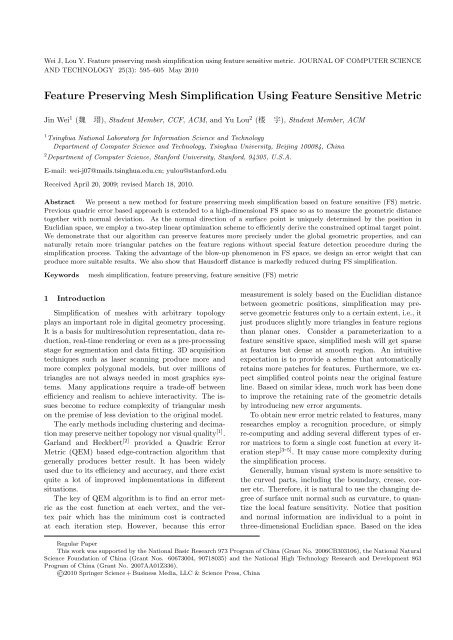
Fig.2. Horse model (10024 tri. to 596 tri.) with green (or red) colored feature region. (a) Input mesh. (b) QSlim result. (c)∼(d) Our
FS method without and with blow-up. The corresponding zoom in viewer are under them, ω = 0.03. Obviously (c) produces more
reasonable result than (b), and (d) preserves more detail for the head rather than retain the triangles on the leg and joints.

Jin Wei et al.: Feature Preserving Mesh Simplification Using Feature Sensitive Metric 597
colors and texture. Having taken note of this, a lot of
work has been proposed over how to enrich the definition
of the error metric with the other information.
Garland and Heckbert [2] introduce surface attribute
and convert the mesh into a high-dimensional space
that is constructed by the positions and colors, then
they measure the distance from an n-dimensional point
to corresponding n-D hyperplane. Hoppe [3] extended
this method to a higher-dimensional space that may
combine information including normal, color and texture
coordinates. He projected each point into attribute
space for measurement. This is equivalent to construct
a combined error metric. In addition, Cohen et al. [10]
designed a texture coordinate related simplification approach
that reduces the distortion for texture mapped
models. Since then, the research about feature preserve
contraction has become to propose a new combination
of the error matrices, such as [4 - 5]. Moreover some direct
methods such as [11] are proposed to preserve feature
as the user specifies by UI input. Garland [12] summarized
the method based on high-dimensional space
and extends to arbitrary manifold. In addition, attribute
analysis is also introduced in order to preserve
pre-detected features such as [4,13 - 14] . Based on the exactly
extracted feature lines, these methods extended
QEM into a weighted quadric metric, vertices close to
feature line get a large weight so that they are hard to
eliminate. Moreover, rather than finding a local minimization
in [2 - 3, 12], [15] proposed a variational approach
to computing the simplified mesh under global
optimization method, in which the metric in [2] was
extended to processing mesh normals. This method is
good to capture anisotropy and also to reduce the geometric
errors.
3 Simplification in FS Space
In this section, we will discuss the details of our proposed
algorithm. The overall pipeline of the algorithm
is first presented. Quadric error matrix extended in
FS space is then discussed in detail. We finally give an
algorithm to compute the optimized position. Since position
and normal at each vertex is not freely separated,
we introduce an optimization based algorithm to find
the optimal vertex position in replace of an contracted
edge.
3.1 Algorithm Overview
QEM based method is generally a “Selection-
Contraction” iteration process. In three-dimensional
Euclidian space, quadric metric that indicate the sum
of squared distance from a space point to its correlative
adjacent plane can be converted into a 4 × 4 symmetric
matrix under homogeneous coordinates. It is in fact
the discrete form of TDM (Tangent Distance Minimization)
from the space point to the vertex of the current
valid pair.
In FS space, we describe a six-dimensional vector as
v i = (p i , wn i ), where p i and n i indicate its position
and normal in R 3 respectively, while w is the feature
sensitivity weight as defined in the previous section. Its
error matrix Q i is then extended to a 6 × 6 symmetric
matrix. Following the principle proposed in [2], the
matrix form of discrete squared tangent-point distance
in FS space
ε i (v) = (v − v i ) T Q i (v − v i ) (1)
is defined to be the contraction error for each vertex
v i , and the cost of the k-th contraction (v i , v j ) → ¯v is
similarly chosen to be ξ k (¯v) = ε i (¯v) + ε j (¯v).
In order to preserve feature more precisely, the best
choice to derive contraction target point is to find an optimal
vertex ¯v that minimizes the error function ξ k (¯v).
Notice that ξ k (¯v) is now an energy function defined in
FS space, the main difference to R 3 is that optimization
in FS space is in fact a constrained optimization
problem. In Subsection 3.2, we introduce an efficient
constraint iteration scheme to fast obtain the optimized
target point under FS error metric.
Now we could give a summary of our FS simplification
algorithm as follows. Selection of valid pairs have
been done during initialization and the selection rules
are similar as described in [2]. As we map unit normal
vector for each vertex with a non-negative w, in order
to produce uniform effects for this quantity on different
models, we simply fitted all models into a unit cube
before FS mapping, and rescale back after the simplification.
In this paper, we set w = 0.03 expect for
specific statement.
Input: polygonal mesh in FS space.
Output: simplified mesh with more triangles remaining
in the feature regions.
Algorithm:
1) For each vertex, compute the 6 × 6 FS error matrix
Q i .
2) For each valid pair, compute the target point
(v i, v j) → ¯v that minimizes the constrained cost
function ξ k (¯v) = ε i(¯v)+ε j(¯v); push every valid pairs
into a minimum-heap according to the quantity of
ξ k (¯v).
3) Contract a vertex pair which is the top element in the
heap, update the error for each new adjacent vertices
as 2, iterate until the target amount of triangles is
achieved.
4) Post cleaning (Optional).
Note that the input mesh is a polygonal mesh
mapped to FS space. It may have blow-up phenomenon

598 J. Comput. Sci. & Technol., May 2010, Vol.25, No.3
about feature line [8] . This may cause some singular
problem during the process because they have identical
position vector in R 3 . The treatments for blow-up
region are discussed in Section 4.
3.2 Derive Quadric Matrix in FS Space
Definition of the cost function is a pacing factor for
visual effect. It is noticed that a mesh in FS space is actually
a 2-manifold embed in R 6 . FS space is therefore
a non-free form space that is constrained by the geometric
properties and topology in three-dimensional
Euclidian space. Because the input model is existing in
R 3 in essence, operations in FS space must satisfy the
space restriction. Error measurements is then defined
from R 6 to original R 3 . Previous works have chosen to
use the discrete approximation of the tangent plane at
a mesh vertex. Here we map the planes of the triangles
that meet at the original vertex in R 3 onto a 2-d hyperplane
embed in R 6 to approximate the corresponding
tangent space. The contraction cost is then defined by
the squared distance between the space point and that
2-d hyperplane.
As we have three given points lying on the triangle
that are mapped from R 3 , one can always get two edge
vectors e 1 and e 2 in R 6 . Then, for a six-dimensional
element v, evaluating the distance to the 2-hyperplane
which determined by this triangle is essentially equivalent
to finding the nearest point v min in the linear
subspace W that is spanned by e 1 and e 2 :
d 2 i = min‖v − v t ‖ 2 , v t ∈ W (2)
The squared distance from an arbitrary vertex v in FS
space to the subspace W is now established as:
d 2 i = v 2 ⊥
= (v − v i ) T K T K(v − v i )
= (v − v i ) T K(v − v i ). (7)
Thus the error metric for v i can be easily derived in an
additional form:
ε i (v) = ∑ d 2 i
= ∑ (v − v i ) T K i (v − v i )
= (v − v i ) T ∑ K i (v − v i )
= (v − v i ) T Q i (v − v i ) (8)
where Q i is set to be the error matrix of v i . Similar to
the previous works, we suggest using homogenous form
to represent ε i , thus the updated error of new contract
point can simply become an additional form.
3.3 Contraction Point Optimization
Edge contraction can be treated as an iteration process.
Although we can simply choose the target position
as v i , v j or their midpoint, to preserve geometric details
as much as possible, the best choice is to estimate an
optimized location that minimizes the six-dimensional
quadric error with the geometric constraint in R 3 .
where v t is an arbitrary vertex in W . To this end, we
aimed to finding a vector v ⊥ = v − v min − v i which
is orthogonal to the linear subspace W with its origin
at v i . Let us define a 2 × 6 matrix A = [e 1 e 2 ] T and
local coordinates x min on the basis of the subspace, i.e.,
v min = A T x min + v i . We could now set an equation as:
A(v − A T x min − v i ) = 0. (3)
Solving (3) w.r.t. x min , we derived that
So that
v min = A T (AA T ) −1 A(v − v i ). (4)
v ⊥ = v − v min − v i
= (I − A T (AA T ) −1 A)(v − v i )
= K(v − v i ). (5)
Obviously, K is a 6 × 6 symmetric matrix. Moreover,
we also noticed that K is implicitly comprised of the
Moore-Penrose inversion of A. Therefore, K can be
rewritten as K = I − A + A, such a matrix is idempotent:
K 2 = K T K = K. (6)
Fig.3.
Comparison with non-constraint optimization in FS
space. (a) Original mesh. (b) Our method. (c) Modified QEM
method [12] .
Note that in FS space, vertex is combined by its
position and weighted normal in R 3 . Once a position
in R 3 has been set, the attached normal vector will
be uniquely determined by its local geometry. Due to
this restriction, solving the minimization problem directly
in FS space without constraint may lead to unexpectable
result (see Fig.3). Therefore we propose an
iteration scheme with linear search and an initial guess
v i = (p i , ωn i ) to derive a constrained optimization target
point in FS space. The flowchart of this optimization
procedure is shown in Fig.4.

Jin Wei et al.: Feature Preserving Mesh Simplification Using Feature Sensitive Metric 599
Fig.4. Flowchart of the constrained optimization procedure for deriving target contraction point.
In case we obtain an optimized position p ′ i with a
fixed normal n ′ i , the corresponding normal n′ i for this
local optimization position could be derived by its local
geometry.
Notice that as the step factor t can strictly reduce
the quadric error during each iteration step, the optimization
is guaranteed to be a convergent procedure.
To assign an initial value, we get optimized p i+1 under
fixed n mid that derived from the average of two original
normals. The corresponding normal vector n i+1
is then evaluated by the revised local geometry. According
to Subsection 3.1, cost function is defined to
be a quadratic form, so that searching between initial
point and optimized point is a linear problem. In our
experiments, we have found out that most iteration will
be done within 2∼4 times. Fig.5 shows the results using
linear search iteration in different times, searching
within 4 times provides acceptable effects.
4.1 Error Weights for Blow-Up Regions
It is claimed that the input of our algorithm is a
polygonal mesh in FS space. In the theory of featuresensitive
geometry processing, one can generate blowup
regions for sharp feature when the inner product
of two face normals is greater than a user defined
threshold, so as to possess further area in parameter
domain [8] . Such blow-up points which have identical
positions but dissimilar normal directions in R 6 are essentially
the same in the three-dimensional Euclidian
space. Simplification without special rules may result
in unexpectable mistake about feature region. As described
in [8], blow-up phenomenon expand the area
of features in parameter domain, so that the result of
parametrization is well improved. However, as the more
we assign feature sensitivity, the more points would be
generated in FS space. In Fig.6, blow-up vertices explicitly
decompose the variation of the normal direction
Fig.5. Target point optimization with 1-time (see (b)) and 4-
time (see (c)) iterations for each new vertex. (c) produces more
suitable result.
4 Additional Details to Geometric
Optimization
In this section, we give further details to some steps
of the pipeline, including dealing with blow-up regions,
and the post cleaning operation.
Fig.6. The blow-up phenomenon at sharp edges and corners. (a)
Original mesh in R 3 . (b) Projection of the corresponding mesh
in R 6 . Normal vectors are set to be the face normals on the two
sides of the edge and the interpolation between them.

600 J. Comput. Sci. & Technol., May 2010, Vol.25, No.3
on creases and corners. It means that vertices in feature
regions in FS space have tiny difference only at the
coefficients related to normal direction. When a vertex
on sharp feature is decomposed into several new points
in FS space, features will get flatter than their preimage
in R 3 , so that contraction error in blow-up regions will
be extremely small. This indicates that sharp features
which have been blown will get top priority in the error
heap. To avoid this, the number of blow-up vertex
have to be constrained. We have found out that most
feature vertices can at most be decomposed into two
or three 6D points, and the improvement under this
strategy could be ignored. This may lose the advantages
of both the error metric in FS space and blow-up
phenomenon.
For this reason, a specific rule that simulates the effect
of blow-up scheme is designed. The basic idea is
to change the contraction cost function into a weighted
quadric error rather than veritably expands the features
into several blow-up points which are identical
in R 3 . The weighted quadric error is then defined as:
ξ
k ′ = η kξ k where η denotes the number of vertices that
the current vertex will be expanded to. We firstly
launch a shrink-back procedure during initialization to
ensure there is no degenerated edge in R 3 . The blow-up
weight is then directly inherited from the blow-up rule
in [8] as follows.
1) If a vertex v is neither labeled as edge nor corner
vertex, we simply set η i = 1.
2) If v lies on the edge which the angle deviation
θ of normal vector on either side of the edge is larger
than a threshold value θ E (we use π/4 for all models in
this paper), this vertex is treated as edge vertex. The
corresponding weight is assigned as:
η i =
⌈ θ
θ t
⌉
+ 1 (9)
According to the above rules, Ση i is obvious with
the same amount of vertices at the blow-up region in FS
space. So this rule will not lose the significance of blowup
phenomenon. To ensure that contraction point is a
local minimum under FS error metric, blow-up weights
should not be taken into account in the optimization.
In other words, η only influences the priority of the
elements in error heap.
The rule for updating error cost of contraction point
¯v is also improved. For a vertex pair with at most one
blow-up vertex, new weight is set to be the average of
η i , η j , so that new error cost equivalent to the general
cases. For a pair containing two vertices that the corresponding
weights are all greater than 1, new weight
for target point is updated to η i + η j , so that error cost
actually becomes (η j + η j )(ξ i + ξ j ), meaning that when
an edge containing two feature vertices is contracted,
the optimized contraction position is an abstraction of
the current feature region, so it should be more difficult
to simplify.
Although this procedure extract feature naively, we
found this strategy gives further improvement to FS
metric based method. Results in Fig.2 demonstrates
the effectiveness of this method.
4.2 Preserving and Post Cleaning
Open boundaries require additional constraint during
the optimization process. For a contraction containing
boundary points v b , linear search for optimization
point is constrained in the plane that is spanned by
two boundary edges intersecting at v b . For simplicity,
we search the optimized boundary point along the
boundary line which consists of v bleft , v b and v bright .
We test face-flipping after target point optimization. In
case that flipping occurred, we use a penalty multiple to
where “⌈·⌉” denotes the ceil operation, θ t is an userspecified
step factor means the mesh density in blow-up
region.
3) If there are at least three sharp edges meeting at
a vertex, this vertex is treated as a corner. Moreover,
a cone-like vertex is also labeled as corner if the sum of
the angle of one-ring neighboring triangles is less than
2π cos θ C , where θ C is the corner threshold, we use π/12
in this paper. Blow-up weight for corners is then defined
as:
η i = ∑ η k + 1 (10)
where η k is the weight of the k-th neighbor vertex of
the corner v. For simplicity, we do not allow the existence
of the two adjacent corners. Once it occurs, we
use a dummy point between them and simply set it as
an edge point.
Fig.7. Edge-flipping to remove near-degenerated triangles. (a)
Before edge-flipping. (b) After edge-flipping. The amount of
faces is not changed after the flipping process.

Jin Wei et al.: Feature Preserving Mesh Simplification Using Feature Sensitive Metric 601
increase their contraction cost. In our experiments, we
always use 3 for penalty.
Because this algorithm is based on a feature sensitive
metric, sharp features will hold more triangular
patches but less triangles to represent planar regions.
In many cases, remaining triangles get narrower than
another QEM based method. For very few triangles
that consist of planar points and near-feature points, it
may become narrow or degenerated triangles through
the optimization under FS error metric. Consider that
narrow triangles may give instabilities to the follow-up
processing, we employ an edge-flipping (as Fig.7) treatment
to remove degenerated triangles if it satisfies the
inequality as:
|edge k + edge (k−1) | − |edge (k+1) | < τ (11)
where k = 0, 1, 2, τ is a small positive floating number
less than 1 (we set as 10 −4 ). Obviously, this treatment
does not alter the amount of remaining faces.
5 Results and Discussions
We have proposed a feature sensitive simplification
approach running in FS space. We have implemented
this method to investigate with widely used quadric
error based simplification framework, QSlim. We compare
the results form the visual qualities and statistical
analysis of the produced errors (in Fig.8). All test models
has distinct feature regions including creases, corners
and boundaries as in Figs. 2, 9, 10 and 11, these
results demonstrated our method can preserve feature
more precisely.
For a simplified mesh, remaining vertices on the planar
regions can be treated as redundancy. We have
the first impression with Fig.9 that our algorithm retains
more patches on the feature region to eliminate
the redundant information. To quantize this ability,
many criteria can be met, such as [16 - 17]. In this
paper we just use the well-known two-sided Hausdorff
distance measurement tool, Metro, as designed in [17]
for evaluating mesh quality, to compare the similarity
between simplified and original models. In addition,
because our algorithm is defined in FS space, we also
measure a six-dimensional Hausdorff distance that is
defined to be the Euclidian distance from an FS space
point to a embedded two-dimensional triangle patch, in
order to deal with the effectiveness of error optimization
in FS space. To avoid ambiguities we call the Hausdorff
distance defined in R 3 and R 6 as geometric error and
FS error (or distance) respectively.
Fig.8 shows some quantified results during experiments
with simplification of Lucy model. We observed
that FS metric based method produces a significant improvement
on geometric error than QSlim. That is,
as the traditional quadric errors are not defined in a
feature-isotropic space, distortions may be caused when
a large data reduction occurred. If we apply the algorithm
to simplify massive meshes, tiny errors will accumulate
with the increasing of reduction percentage during
the simplification process (see Fig.8(a)). Although
we calculate optimized solution for contraction at each
step, this may still introduce some adverse effects on
the visual quality. We know that Hausdorff distance
defined in R 3 indicates max geometric error between
two given models, and large errors are caused when the
edge containing feature point is collapsed. Intuitively,
human vision system is sensitive to contours and sharp
regions. As shown in Fig.8(d), our method preserves
the contour of Lucy model and then naturally assigns
more triangular patches on the regions with large normal
variations. This effect is useful especially when we
take a large reduction rate. For this reason, FS method
provided preferable results, and, as more feature points
are retained, geometric error is greatly reduced compared
with QSlim as shown in Fig.8(a).
Fig.8. Quantized produced errors during simplification of Lucy model (c). Errors are classified into two categories as Hausdorff distances
in R 3 (a) and R 6 (b). (d) Zoom in image of details on the simplified models using QSlim (left) and FS (right). Our method gets high
visual quality on the details.

602 J. Comput. Sci. & Technol., May 2010, Vol.25, No.3
Moreover, we also interested in the Hausdorff distances
in FS space. In Fig.8(b), we found that statistical
results did not provide remarkable contrast in
different stages, but FS method got a steadier error
curve and is well constrained under 20%. This is
reasonable because the optimization discussed in Section
3 did not make a globally optimized solution,
but a constrained local minimum. However, as these
constrained-optimized points are derived with an userspecified
threshold value uniformly, the overall FS error
can be kept within a bound.
In another similar result shown in Fig.9(a), we found
that FS method provides a dense approximation for facial
features but large triangles on the planar regions
like forehead and cheeks. Fig.9(b) also shows that more
patches are assigned and retained on the sharp features,
but fewer samples are remained on the planar regions
under the same reduction rate. This effect is useful for
a smooth shading effect on important regions.
In Subsection 4.1, we described the benefits of blowup
phenomenon to parametrization. Here we discuss
the effects of this strategy in mesh simplification. As
we mentioned, blow-up strategy is a naive feature
extraction that simply inspects the angular distance
between two adjacent face normals. Although some
feature extraction based method as [14] provides robust
and convincing results, they still have to compute
distance from each vertex of the mesh to the nearest
feature point to set global costs. So, result quality of
feature extraction based method depends on the quality
of extracted feature line. Then, one may spend much
time to select an appropriate argument for different input
models in different detection scales. The advantage
of blow-up weight strategy is that it is quite simple and
easy to compute. Instead of tracking an exact feature
line, the definition of blow-up weight aims to simulate a
uniform point sampling in FS space, and, as we saw in
Figs. 2 and 10, this strategy can give a noticeable improvement
to a flat FS metric based approach. Those
results show that details on the ears of the horse and
facial features on the Leopard model may be thrown
off instead of remaining during QSlim procedure. It is
clearly shown that FS method produces more suitable
results for global features especially on head and claws.
However, we noticed that some unimportant features
like joints and legs have taken excessive patches over
Fig.9. Contrast of two models between QEM (center) and FS (right). (a) LittleThinking (400K tri. to 7.4K tri.). (b) RockerArm
(80K tri. to 6K tri.). Sharp features are tagged in green color. Red cubes are tagged on some feature regions, and the regions are
approximated by more triangles than QEM.
Fig.10. Leopard model (65 024 tri. to 996 tri.) with green (or red) colored feature region. (a) Initial model. (b) Result of QSlim.
(c)∼(d) FS method without and with blow-up, and their zoom in viewer under them, ω = 0.03. We see FS method preserves the
contour and facial features are completely preserved by FS with blow-up.

Jin Wei et al.: Feature Preserving Mesh Simplification Using Feature Sensitive Metric 603
Table 1. Quantization of Max/RMS Errors (The minimum errors are labeled in bold.)
Models (remaining%) Types QSlim FS FS with Blow-Up
LittleThinking (1.8%) R 3 0.008 774/0.000 874 0.005 226/0.000 971 –
R 6 0.012 617/0.003 097 0.014 436/0.003 109 –
RockerArm (7.5%) R 3 0.007 141/0.000 622 0.003 717/0.000 509 –
R 6 0.016 153/0.004 979 0.020 003/0.004 491 –
Horse (6.0%) R 3 0.029 360/0.005 777 0.019 573/0.005 392 0.026 271/0.006 531
R 6 0.026 384/0.012 863 0.022 827/0.011 269 0.028 869/0.011 024
Leopard (1.5%) R 3 0.031 569/0.007 015 0.014 799/0.003 223 0.025 460/0.004 342
R 6 0.033 461/0.011 183 0.022 460/0.008 569 0.022 437/0.008 740
HappyBudda(6.5%) R 3 0.012 378/0.001 195 0.010 627/0.001 891 0.011 453/0.001 824
R 6 0.020 172/0.005 973 0.019 132/0.006 245 0.022 634/0.006 240
simplified model rather than assigned on the head
(Fig.2 bottom), because joints may consist of many
small triangles in original model so that the geometric
variance near the joints may be larger than which
is on the head. Similarly, eyes were also eliminated on
the simplified Leopard model. Although for textured
models, these results derived by standard FS method
are sufficient for most applications. One may still prefer
to get a more compact abstraction that preserve
most of main facial features. To achieve this goal, we
may introduce the blow-up weight strategy. Fig.2(d)
and Fig.10(d) show the results produced by weighted
FS method. For the same number of remaining triangles
and blow-up arguments, facial features are approximated
by more patches but little on legs and tails.
Visual effects for both models got good enhancements.
These results have demonstrated our weight strategy is
effective and easy to use. It is useful when users have
to face to a large database.
It is noticed that having more triangles on features
means remaining less on the planar regions. The more
features are remained, the larger the error will be introduced
in planar regions. On the other hand, QEM
method uses a geometric error-driven greedy optimization,
all the target vertex is derived under least-squared
sense, so that to deal with RMS (Root Mean Squared)
errors, FS method does not provide remarkable improvement.
Table 1 lists error comparisons for all example
models used in this paper, with its remaining rate
correspondingly. We see that for FS methods, most
RMS errors are smaller, but QSlim outperforms occasionally.
On the other hand, for weighted FS method,
though most of remaining feature points are preserved,
RMS error may still exceed QSlim because the planar
regions are approximated by the triangles that are even
larger than a flat FS method. But we claim that as FS
methods get much lower maximum errors, FS methods
make much better outputs for visual effect. So these
results are much more useful than those derived by QSlim.
Another example of HappyBudda model is shown
in Fig.11. The corresponding errors are also listed in
Table 1. We see that although QSlim outperforms our
method on RMS error, features (marked as green color
in Fig.11(a)) are preserved much better by FS. When
the blow-up weight is applied, details of remaining features
are superior to flat FS method.
It is notable that reasonable arguments for feature
sensitivity will give different distributions of triangles
Fig.11. HappyBudda model (123 056 tri. to 8 032 tri.) with feature region colored in green or red. (a) Initial mesh. (b) QSlim result.
(c)∼(d) FS method without and with blow-up. Their zoom in images are shown in (e) in the order.

604 J. Comput. Sci. & Technol., May 2010, Vol.25, No.3
Fig.12. Simplifying Ateneam model with various feature sensitivity arguments, 15 104 to 1 992 tri.: All simplified models is derived by
FS method without blow-up, ω is set as 0, 0.01, 0.03, 0.1, 0.3. If ω is set to 0, the result is similar to the previous QEM method. When
ω is upgraded, more triangles are retained on the sharp edges but distortion is also occurred at the planar regions.
for simplified mesh. Fig.12 shows a series of simplified
Ateneam models with different w in ascending order.
We see the facial features are approximated by
further patches under larger weights. However, large
weight may cause too large distortions on planar regions.
When w is upgraded to 0.3, though the details
of eyes and mouth are preserved well, the overall appearance
of facial form becomes unacceptable.
Although our inception is focused on the accuracy
but is not efficiency during simplification, we are still
concerned about performance. A direct speculation is
that, as FS methods take more dimensions into account,
and iterate at each step, we have to cost more time
than QEM method. We implemented our method and
QSlim is also integrated into the same testing framework,
comparing the performance for both methods on
a laptop with Intel Duo 2.5 GHz processor and 2 GB
main memory. Table 2 shows the comparison results
for each model used in this paper. Our approach costs
around double times than QSlim in most cases. This is
an limitation of FS method that there exists a tradeoff
between appearance, speed and interactivity, but it
is still faster than some other appearance preserving
based method like [15], that is mentioned as three to
twenty times slower than QEM. For fair comparison, we
do not introduce any special scheme for acceleration, so
there are quite a lot strategies which can be employed
for further improvement, e.g., using vertex heap rather
than edge heap [18] . The performance of FS method is
also related to the input quality, for the reason that a
complex model may bring more iteration steps.
Table 2. Time Comparison (in ms)
Models No. Faces QSlim FS
Horse 10 024 180 312
Leopard 65 024 1 224 2 612
RockerArm 80 354 1 650 3 129
HappyBudda 123 056 2 663 4 922
Lucy 237 278 5 399 9 871
LittleThinking 401 985 8 249 17 463
6 Conclusions and Future Work
We have presented a new simplification algorithm
based on FS metric. According to the constraint conditions,
we construct error metric by using the sum of the
squared distance from a 6D point to its corresponding
two-dimensional hyperplane rather than in R 3 . Moreover,
we employed a constrained optimization to acquire
contraction target point which satisfies the geometric
constraint on normal directions, this strategy
may also be combined with other normal-geometry related
cases. Experimental results demonstrated that
this algorithm can preserve feature more precisely under
the global geometry, and then naturally retain more
patches on the feature regions without special feature
recognitions during the simplification process.
Taking the advantage of blow-up phenomenon in FS
space, our method can produce more suitable result and
high visual quality on feature regions.
However, as we have known that the tradeoff between
efficiency and accuracy has become the bottleneck
to simplification, feature sensitive simplification
with the high-performance computing technology may
become a significative research topic.
References
[1] Heckbert P, Garland M. Survey of polygonal surface simplification
algorithms. In SIGGRAPH 1997 Course Notes: Multiresolution
Surface Modeling, 1997.
[2] Garland M, Heckbert P. Surface simplification using quadric
error metrics. In Proc. SIGGRAPH, Los Angeles, USA,
Aug. 3-8, 1997, pp.209-216.
[3] Hoppe H. New quadric metric for simplifying meshes with
appearance attributes. In Proc. the 10th IEEE Visualization
Conference, San Francisco, USA, Oct. 24-29, 1999, pp.59-66.
[4] Yan J, Shi P, Zhang D. Mesh simplification with hierarchical
shape analysis and iterative edge contraction. IEEE Transactions
on Visualization and Computer Graphics, 2004, 10(2):
142-151.
[5] Jong B S, Teng J L, Yang W H. An efficient and low-error
mesh simplification method based on torsion detection. The
Visual Computer, 2005, 22(1): 56-67.
[6] Kimmel R, Malladi R, Sochen N. Image as embedded maps
and minimal surfaces: Movies, color, texture and volumetric
medical images. International Journal of Computer Vision,
2000, 39(2): 111-129.

Jin Wei et al.: Feature Preserving Mesh Simplification Using Feature Sensitive Metric 605
[7] Lai Y K, Zhou Q Y, Hu S M, Wallner J, Pottmann H. Robust
feature classification and editing. IEEE Transactions on
Visualization and Computer Graphics, 2007, 13(1): 34-45.
[8] Lai Y K, Hu S M, Pottmann H. Surface fitting based on a
feature sensitive parameterization. Computer-Aided Design,
2006, 38(7): 800-807.
[9] Lai Y K, Zhou Q Y, Hu S M, Martin R R. Feature sensitive
mesh segmentation. In Proc. ACM Symposium on Solid and
Physical Modeling, Cardiff, UK, June 6-8, 2006, pp.17-25.
[10] Cohen J, Olano M, Manocha D. Appearance-preserving simplification.
In Proc. the 25th Annual Conference on Computer
Graphics and Interactive Techniques, Orlando, USA,
July 19-24, 1998, pp.115-122.
[11] Kho Y, Garland M. User-guided simplification. In Proc.
ACM Symposium on Interactive 3D Graphics, Monterey,
USA, April 27-30, 2003, pp.123-126.
[12] Garland M, Zhou Y. Quadric-based simplification in any dimension.
ACM Transactions on Graphics, 2005, 24(2): 209-
239.
[13] Lindstrom P, Turk G. Image-driven simplification. ACM
Transactions on Graphics, 2000, 19(3): 204-241.
[14] Yoshizawa S, Belyaev A G, Seidel H P. Fast and robust detection
of crest lines on meshes. In Proc. ACM Symposium on
Solid and Physical Modeling, Cambridge, USA, June 13-15,
2005, pp.13-15.
[15] Cohen-Steiner D, Alliez P, Desbrun M. Variational shape approximation.
In Proc. ACM SIGGRAPH, Los Angeles, USA,
Aug. 8-12,, 2004 pp.905-914.
[16] Bian Z, Hu S M, Martin R R. Evaluation for small visual difference
between conforming meshes on strain field. Journal
of Computer Science and Technology, 2009, 24(1): 65-75.
[17] Cignoni P, Rocchini C, Scopigno R. Metro: Measuring error
on simplified surfaces. Computer Graphics Forum, 1998,
17(2): 167-174.
[18] Hussain M. Efficient simplification methods for generating
high quality LODs of 3D meshes. Journal of Computer Science
and Technology, 2009, 24(3): 604-inside back cover.
Jin Wei is a Master candidate
at the Department of Computer Science
and Technology, Tsinghua University.
His research interests include
digital geometry processing, video
processing, and computational camera.
He is a student member of China
Computer Federation and ACM.
Yu Lou is currently a Master
candidate in the Department of Computer
Science, Stanford University.
His research interests include computer
graphics, mesh processing, and
image processing. He is a student
member of ACM.