A Spiking Neuron Model for Binocular Rivalry - Psychology

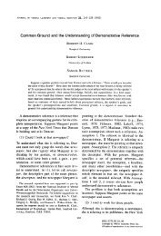
Journal of Computational Neuroscience 12, 39–53, 2002
c○ 2002 Kluwer Academic Publishers. Manufactured in The Netherlands.
A Spiking Neuron Model for Binocular Rivalry
CARLO R. LAING
Department of Mathematics, University of Pittsburgh, Pittsburgh, PA 15260, USA; Department of Physics,
University of Ottawa, 150 Louis Pasteur, Ottawa, Ontario, Canada K1N 6N5
claing@science.uottawa.ca
CARSON C. CHOW
Department of Mathematics, University of Pittsburgh, Pittsburgh, PA 15260, USA
ccc@math.pitt.edu
Received November 27, 2000; Revised October 26, 2001; Accepted November 29, 2001
Action Editor: Kenneth D. Miller
Abstract. We present a biologically plausible model of binocular rivalry consisting of a network of Hodgkin-
Huxley type neurons. Our model accounts for the experimentally and psychophysically observed phenomena: (1) it
reproduces the distribution of dominance durations seen in both humans and primates, (2) it exhibits a lack of
correlation between lengths of successive dominance durations, (3) variation of stimulus strength to one eye influences
only the mean dominance duration of the contralateral eye, not the mean dominance duration of the ipsilateral
eye, (4) increasing both stimuli strengths in parallel decreases the mean dominance durations. We have also derived
a reduced population rate model from our spiking model from which explicit expressions for the dependence of
the dominance durations on input strengths are analytically calculated. We also use this reduced model to derive an
expression for the distribution of dominance durations seen within an individual.
Keywords:
binocular rivalry, multistable perception, visual perception
1. Introduction
Binocular rivalry occurs when the two eyes are presented
with drastically different images. Only one of
the images is perceived at a given time, and every
few seconds there is alternation between the perceived
images. The perceived durations of the images are
stochastic and uncorrelated with previous perceived
durations (Fox and Herrmann, 1967; Walker, 1975).
Also, changing the contrast of the images will change
the dominance durations of the perceptions in specific
ways.
It is not yet clear exactly what is rivaling during
binocular rivalry (Lee and Blake, 1999; Logothetis
et al., 1996). It was traditionally thought that the rivalry
was between the two eyes (Blake, 1989; Lehky, 1988).
However, there is more recent evidence that the neurons
at the site(s) of rivalry have access to information
from both eyes (Carlson and He, 2000; Kovacs et al.,
1996; Lumer et al., 1998; Ngo et al., 2000), and these
experimental results cannot be explained in terms of
“eye rivalry” (although see Lee and Blake, 1999, for
an indication of how changing stimulus characteristics
can produce either “eye rivalry” or “stimulus rivalry”).
Recordings in the cortex of monkeys undergoing
binocular rivalry indicate that the neuronal activity
of binocular rather than monocular neurons is
correlated with the perception of one of the presented
images (Leopold and Logothetis, 1996, 1999;
Logothetis, 1998; Logothetis et al., 1996; Logothetis

40 Laing and Chow
and Schall, 1989). The proportion of neurons that are
active only when one of the images is perceived increases
as one moves up the visual pathway (Leopold
and Logothetis, 1999; Logothetis, 1998). It should be
noted that while some neurons are more active when
their preferred image is perceived, others are more active
when their preferred image is suppressed, and yet
others show little selectivity during nonrivalrous stimulation
but become more selective during rivalrous stimulation
(Leopold and Logothetis, 1996; Logothetis,
1998; Logothetis and Schall, 1989).
Several explanations of binocular rivalry have been
proposed (Dayan, 1998; Gomez et al., 1995; Lehky,
1988; Lumer, 1998). One set of theories propose that
the alternation is due to some form of reciprocal inhibition
between the two monocular pathways (Blake,
1989; Lehky, 1988). Many of the existing theories involve
neural network or rate models for which making
direct quantitative comparisons with neurophysiological
recordings are not possible.
Our focus is on the specific biophysical mechanisms
responsible for binocular rivalry and multistable perception.
We present a network of Hodgkin-Huxley-type
neurons that reproduces the observed psychophysical
and experimental behavior. Our network consists of
both excitatory and inhibitory cells in a biophysically
plausible cortical network. We then present a reduced
population rate model derived from the spiking neuronal
network. We propose that the known observed
phenomena associated with binocular rivalry are direct
consequences of the underlying physiology of coupled
spiking neurons.
We propose that a given percept is represented
as a localized focus of active neurons (Hansel and
Sompolinsky, 1998; Laing and Chow, 2001). In the
simple case of the two presented images being oriented
gratings (Lee and Blake, 1999; Logothetis et al., 1996),
we suggest that a population of neurons is tuned to a
given orientation, and neurons in this population are locally
connected to other neurons with similar preferred
orientations. (We note that our spiking model could
be adapted so that the two foci represent eye images.)
When a grating of a given orientation is presented,
the network receives orientation-specific inputs, and
the local cortical connectivity shapes the activity of the
population to fire maximally at the preferred orientation
with a drop off in activity away from the maximum
in a way that matches the tuning curve of the individual
neurons. One possibility is that this network is situated
at a higher-level visual area, where inputs arrive both
from lower level visual areas and from higher-level
cortical areas.
When two conflicting stimuli are presented, the network
is unable to sustain activity centered around
both inputs simultaneously and thus alternates between
one focus of activity and the other. This switching is
the neurophysiological correlate of binocular rivalry.
The switching is induced by a slow process such as
spike frequency adaptation or synaptic depression. The
dominance duration depends on not only the time scale
of the slow process but also strongly on the input
strength to the network. This allows for large variations
in the dominance times even when the time-constant of
the slow process is fixed. Our simulations and analysis
show that the behavior of the network matches the
observed behavior in a number of ways: (1) it reproduces
the distribution of dominance durations seen in
humans and primates, (2) there is a lack of correlation
between lengths of successive dominance durations,
(3) variation of stimulus strength to one eye influences
only the mean dominance duration of the contralateral
eye, not the mean dominance duration of the ipsilateral
eye, (4) increasing both stimuli strengths in
parallel decreases the mean dominance durations, and
(5) rotating the bars so they are no longer orthogonal
increases mean dominance durations. The model’s behavior
when the stimulus strength to one eye is changed
in synchronization with either the suppression or dominance
of the percept presented to that eye also agree
with experimentally observed behavior.
Our model combines local cortical circuits and
higher-level control to explain binocular rivalry. Local
cortical circuits are responsible for selecting which
neurons are involved in the particular perception and
inducing the switching between the alternate perceptions.
High-level feedback can play a role in setting
the eventual mean dominance times and can strongly
influence which image is perceived.
2. Hodgkin-Huxley Type Model
Our model consists of a network of excitatory and
inhibitory Hodgkin-Huxley-type conductance-based
neurons in a biophysical cortical network architecture.
The neurons are orientation selective and receive external
inputs from both eyes and possibly feedback from
higher levels. They have a “preferred orientation” and
fire at a high rate when presented with a grating at
that orientation. To model the experiment in which the

A Spiking Neuron Model for Binocular Rivalry 41
two eyes are presented with orthogonal gratings, we
inject currents at two locations in the network centered
around neurons whose preferred orientations differ by
90 degrees. The spatial structure of the current input is
Gaussian (see Fig. 1 and Eq. (20)). Note that since
there is no eye-specific information in the network,
this model is also appropriate for the study of monocular
viewing of orthogonal sinusoidal gratings (Andrews
and Purves, 1997; Walker, 1976). In these experiments,
periods of mixed perception are intermingled with periods
of exclusive visibility of one or the other pattern.
We assume that excitatory cells are synaptically coupled
to other excitatory cells with a strength that decays
as a Gaussian function of the difference between
their preferred orientations. There is also coupling with
a Gaussian footprint from excitatory neurons to inhibitory
neurons, between inhibitory neurons, and from
inhibitory neurons to excitatory neurons, with the variable
always being the difference in preferred orientations.
The equations and parameter values are given in
the Methods section.
We include two slow processes. The first is spike
frequency adaptation due to a calcium-dependent
potassium current (Huguenard and McCormick, 1992;
McCormick and Huguenard, 1992). This is sufficient
to cause oscillations in the network’s activity, although
they occur on a similar time-scale to the time constant
of the decay of this current, ∼80 ms. We also include
synaptic depression in the excitatory to excitatory connections
that has a larger time-constant (Abbott et al.,
1997). We find that synaptic depression alone is not
sufficient to cause switching: we need a slow hyperpolarizing
current as well. The switching phenomenon
is quite robust with respect to the exact strengths and
time-scales of these slow variables.
For simplicity, we explicitly model only those
neurons whose activity increases when their preferred
stimuli are perceived. Those neurons that respond
preferentially when their preferred stimuli are suppressed
may be part of a different circuit that is involved
in suppression of a particular image or eye,
and those whose selectivity changes when the stimulus
is changed from rivalrous to nonrivalrous may
be manifesting the effects of attention on perception
(Leopold and Logothetis, 1996; Logothetis, 1998;
Logothetis and Schall, 1989). Neurons in these last two
classes are not explicitly modeled. Those neurons possibly
involved in suppressing an image are similar to
those that fire when their preferred stimulus is dominant
(both groups fire when one image is suppressed) and
our model could be augmented to include such neurons.
2.1. Simulation Results
Figure 2 shows a rastergram of the firing events of the
excitatory neurons in the network given two current
Figure 1. Two coupled networks of binocular, orientation-selective
neurons. The neurons are labeled with their preferred orientation in
degrees. Current is injected to two groups of neurons whose preferred
orientations differ by 90 degrees.
Figure 2. Activity in the excitatory population as a function of time.
The current stimuli are centered at neurons 15 and 45. The right plot
shows detail of the left plot.

42 Laing and Chow
stimuli centered at neurons whose preferred orientations
differ by 90 degrees. At every moment in time,
the activity is localized into a bump that is centered at
either of the two locations of maximum external current
input. A bump in one of these locations is thought
to represent a perception of bars of the corresponding
orientation. The inhibitory neuron activity is very similar
although it has a greater angular spread. Note the
wide spread of activity, lasting less than 100 ms, when
the activity initially moves to another location. The decrease
in width after this period is probably due to the
adaptation current saturating. This type of high activity
at the onset of a percept is seen in some neurons
in superior temporal sulcus and inferior temporal cortex
during binocular rivalry (Leopold and Logothetis,
1999; Sheinberg and Logothetis, 1997). Experimentally,
bursting behavior is also seen in some of these
neurons. Replacing some of the fast excitatory synapses
in our model with slower NMDA-type synapses (as
in Wang, 1999) causes neurons in a bump to burst in
an approximately synchronous fashion while active,
rather than fire approximately periodically and asynchronously
(results not shown). The network is capable
of sustaining only one bump at any given time, and
since the neurons are coupled synaptically, the subthreshold
inputs to the currently suppressed bump do
not affect the currently active bump.
Figure 3 shows the voltage trace from a typical neuron
in a bump. Note the slower firing rate at the end of
a firing episode relative to that at the start. This simulation
used a total of 60 excitatory and 60 inhibitory
neurons and had no external noise. Similar switching
behavior is seen when larger numbers of neurons
are used, but we do not show results for these larger
networks because of the prohibitively large amounts of
computer time required for such simulations.
A histogram of dominance durations is shown in
Fig. 4. It is unimodal and skewed, with a long tail
at long durations. Included are fits to the data of a
Gamma function that is commonly (Kovacs et al., 1996;
Logothetis et al., 1996), although not always (Gomez
et al., 1995; Lehky, 1995), fitted to such data, along with
another function Eq. (12) that is derived in Section 3.1.
Figure 5 shows the autocorrelation coefficients for the
data in Fig. 4. The lack of any strong correlation beyond
zero lag is clearly seen, in agreement with observations
(Lehky, 1988, 1995; Logothetis et al., 1996).
The Lathrop statistic (Logothetis et al., 1996), which
measures the correlation between successive values in
a time series, was calculated ( ¯L = 0.977, σ = 0.073,
Figure 3. Voltage of the 38th neuron in Fig. 2. Note the different
horizontal scales in the lower two plots. The apparent difference in
spike heights is a result of plotting voltage at discrete values of time.
Figure 4. The distribution of dominance durations for the Hodgkin-
Huxley model. The solid line is Eq. (12) with parameters γ = 0.0174,
η =−0.0005, κ = 0.0782, τ = 1.1389, and the dashed is a Gamma
distribution with λ = 2.3593 and r = 6.7381, where the Gamma distribution
is f (t) = λ r /Ɣ(r)t r−1 exp(−λt).

A Spiking Neuron Model for Binocular Rivalry 43
Figure 5. Autocorrelation coefficients for the data in Fig. 4.
giving a z value of 0.31), and this confirms the lack of
a significant correlation. A simple explanation for this
lack of correlation in a completely deterministic system
is that the system is chaotic: the maximum Lyapunov
exponent is approximately 40 s −1 . Since typical dominance
durations are much longer than the reciprocal
of this quantity, switching times can be thought of as
resulting from an extreme “undersampling” of the underlying
dynamical system, and successive dominance
durations will not be correlated (Racicot and Longtin,
1997). This interpretation as undersampling also provides
an explanation of the results of Lehky (1995)
who, by analyzing a time series of dominance durations,
concluded that the underlying dynamical system
was not a low-dimensional chaotic attractor. Both
Kalarickal and Marshall (2000) and Lehky (1988) studied
simple models of binocular rivalry that showed
this lack of serial correlation, but both models had
stochastic inputs.
As a result of the spatial structure of both the external
current inputs and the coupling, neurons in the
network have a range of different input currents and
hence fire at different average frequencies (Hansel and
Sompolinsky, 1998; Laing and Chow, 2001). Thus, the
neurons cannot synchronize, and there should not be
any strong correlations between firing times of different
neurons although weak correlations are possible
(Gutkin et al., 2001). As the number of neurons in
the network increases, fluctuations in the synaptic input
to a given neuron should decrease. The observed
nonzero variance of experimentally obtained distributions
is thought to be due to both fluctuations from the
finite number of neurons in the network and synaptic,
channel or external noise.
The switching can be understood heuristically. In
Section 3 we give a more quantitative explanation. Consider
two input stimuli 1 and 2. Connections between
excitatory neurons promote activity centered at
stimulus 1 or 2, while inputs from the inhibitory population
prevent this activity from spreading over the
whole network. This inhibitory activity is also strong
enough to suppress activity at the site corresponding
to the stimulus that is not perceived. (For sufficiently
strong inputs, two bumps may coexist). Suppose that
population 1 is active and 2 is suppressed, and consider
the effects of the slow current responsible for
spike frequency adaptation. This current increases at
site 1 and decreases at site 2 until eventually the adaptation
remaining from activity at site 2 has decreased
sufficiently that the neurons at site 2 are able to fire
again, immediately suppressing the neurons at site 1.
The adaptation current at site 2 then builds up, the adaptation
current at site 1 wears off sufficiently, and the cycle
repeats. A similar argument can be made if synaptic
depression is the cause of the switching: both the recurrent
excitation at site 1 and the inhibition of the neurons
at site 2 weaken, allowing neurons at site 2 to fire and
suppress neurons at site 1.
One well-known aspect of binocular rivalry is that if
the strength of the stimulus to one eye is changed, it is
largely the mean dominance duration of the other eye
that is affected, not the mean dominance duration of
the eye whose stimulus strength is being changed. This
effect is sometimes known as Levelt’s second proposition
(Bossink et al., 1993; Levelt, 1968) and has been
observed many times (Leopold and Logothetis, 1996;
Logothetis et al., 1996; Mueller and Blake, 1989). More
specifically, if the strength of the stimulus to eye 1 is
decreased, the mean dominance duration of eye 2 typically
increases markedly in a nonlinear fashion, while
the mean dominance duration of eye 1 decreases by a
small amount. We performed this experiment with our
model, and the results are shown in Fig. 6 (together
with data from the reduced model that is presented in
Section 3). They agree well with observations, and an
explanation for this behavior is given in Section 3.
Another experiment that has been performed involves
changing the angle between the two sets of bars
presented to the two eyes. It has been observed that
decreasing the angle from 90 degrees causes the mean
dominance durations to increase (Andrews and Purves,
1997). We performed this experiment on our model,
and the results are shown in Fig. 7. The variation is
small (as it is in experiments) (Andrews and Purves,

44 Laing and Chow
Figure 6. A demonstration of Levelt’s second proposition in a spiking
neuron model. The strength of one input was fixedat0.4 and the
other was reduced. × is mean dominance duration for the stimulus
whose strength was decreased, ◦ is mean dominance duration for
the stimulus whose strength was unchanged. Compare with Leopold
and Logothetis (1996, Fig. 1), Logothetis et al. (1996, Fig. 4), or
Mueller and Blake (1989, Fig. 2). Also shown are rescaled dominance
durations from the reduced model (1) through (6) (dashed and
dash-dotted). See text for details.
If these widths were reduced, smaller angular differences
could have been tested, but the total number of
neurons in the network would have then had to be
correspondingly increased, resulting in prohibitively
long simulation times. An explanation for the dependence
of dominance duration on angle between bars is
given in Section 3.
A further experiment of interest is that of Mueller and
Blake (1989). They changed the strength (contrast) of
the stimulus presented to one eye, but the change was
only made during either dominance or suppression of
that image. For example, if the manipulation is synchronized
with dominance of an eye, the contrast of
the image presented to that eye is changed when that
image is reported as being dominant and is returned to
the baseline level when the image is no longer reported
as being dominant. We performed this experiment with
our model, and the results are shown in Fig. 8. The
Figure 7. Variation of mean dominance duration as a function of
the angle between two sets of gratings presented to the two eyes.
Smaller angular differences could not be tested, since for these values
the two bumps “merged.” The bars indicate the standard deviation of
the dominance durations. Compare with Andrews and Purves (1997,
Fig. 4B(i)).
1997) but significant. Smaller angular differences could
not be tested, as this caused the two bumps to “merge”
into one that spanned both input positions. This is due to
the widths of the Gaussians used in coupling neurons.
Figure 8. The effects of changing the strength of one input in the
spiking neuron model, synchronized to either the suppression of that
image (top) or the dominance of that image (bottom), as described
by Mueller and Blake (1989). The strength of one input was fixed at
0.4, and the other was reduced. × is mean dominance duration for
the stimulus whose strength was decreased, ◦ is mean dominance
duration for the stimulus whose strength was unchanged. Compare
with Mueller and Blake (1989, Fig. 4).

A Spiking Neuron Model for Binocular Rivalry 45
results for the case where the stimulus strength is synchronized
with suppression of that image (Fig. 8, top)
are very similar to the situation described above as
Levelt’s second proposition—i.e., if the stimulus
strength is decreased, the dominance duration of the
ipsilateral eye is largely unaffected, but the dominance
duration of the contralateral eye increases markedly
(compare Fig. 8, top, with Fig. 6). The results shown
in this figure agree well with experimental results
(Mueller and Blake, 1989, Fig. 4). The case when the
stimulus strength is synchronized with dominance of
the image is shown in Fig. 8, bottom. It is seen that
decreasing the stimulus strength slightly decreases the
dominance duration of the ipsilateral eye but leaves
the dominance duration of the contralateral eye essentially
unchanged. This is also in good agreement with
experimental results (Mueller and Blake, 1989). An explanation
for this behavior is given in Section 3.
3. Reduced Description
We make our heuristic arguments more precise with a
reduced spatially averaged model. The resulting equations
are similar to the proposed models of Kalarickal
and Marshall (2000), Lehky (1988), Mueller (1990),
and Wilson et al. (2000). In Appendix B we describe
how the following equations can be derived from our
spiking neuronal network. They represent the spatially
averaged dynamics of two populations of Hodgkin-
Huxley-type neurons with recurrent excitation, crossinhibition,
adaptation, and synaptic depression:
du 1
=−u 1 + f (αu 1 g 1 − βu 2 g 2 − a 1 + I 1 )
dt
(1)
du 2
=−u 2 + f (αu 2 g 2 − βu 1 g 1 − a 2 + I 2 )
dt
(2)
da 1
τ a =−a 1 + φ a f (αu 1 g 1 − βu 2 g 2 − a 1 + I 1 )
dt
(3)
da 2
τ a =−a 2 + φ a f (αu 2 g 2 − βu 1 g 1 − a 2 + I 2 )
dt
(4)
dg 1
τ d = 1 − g 1 − g 1 φ d f (αu 1 g 1 − βu 2 g 2 − a 1 + I 1 )
dt
(5)
τ d
dg 2
dt
= 1 − g 2 − g 2 φ d f (αu 2 g 2 − βu 1 g 1 − a 2 + I 2 ),
(6)
where all constants are positive. Here u i represents the
spatially averaged net excitatory activity of each localized
population seen in the simulations of the spiking
neurons (i = 1, 2 labels the percept or “bump”), a i and
g i are the population adaptation and synaptic depression
variables, respectively. We have included synaptic
depression in both the excitatory and inhibitory connections.
While depression is thought to occur in only
excitatory synapses, the inhibitory neurons in the full
spiking model are largely driven by the excitatory population,
and it is the depression in the excitatory to excitatory
connections that leads to this decrease in inhibitory
activity on the time-scale of the depression, so this is
not an unreasonable choice. For simplicity we take the
gain function f to be the Heaviside step function—
i.e., f (x) = 1 for x ≥ 0 and f (x) = 0 for x < 0. The
constants τ a and τ d are the time constants of the adaptation
and synaptic depression, respectively, and are
both assumed to be much larger than 1. A high level of
u i is assumed to be directly correlated with the perception
of image i. The chaotic dynamics of the spiking
network are not represented in these reduced equations.
They could be mimicked by including stochastic forcing
terms.
The dynamics of (1) through (6) are fairly simple
because of the separation of time-scales between the
activities and the slow variables. Depending on the parameters,
the system either oscillates or goes to a steady
state. The only possible steady states are both activities
at zero (both off), both activities at 1 (both on), or one
at 1 and the other at zero (one on) and its mirror image.
For clarity, first consider the case where only adaptation
is active (i.e., g 1 = g 2 = 1 and we ignore Eqs. (5)
and (6)). For the both-off steady state, the variables
satisfy (u 1 , u 2 , a 1 , a 2 ) = (0, 0, 0, 0). For this state to
exist, the total inputs of the gain functions must be
below threshold—i.e., I 1 < 0 and I 2 < 0. For the bothon
fixed state, (u 1 , u 2 , a 1 , a 2 ) = (1, 1,φ a ,φ a ). In this
case, the inputs must be greater than threshold—i.e.,
α − β − φ a + I 1 > 0 and α − β − φ a + I 2 > 0. Thus,
strong inputs or strong excitation is required for the
both-on state. The one-on case has (u 1 , u 2 , a 1 , a 2 ) =
(1, 0,φ a , 0) or its mirror image. This requires α − φ a +
I 1 > 0 and I 2 − β

46 Laing and Chow
Repeating for a 1 we get the same equation but with the
indices reversed. This then allows us to solve for T 1
and T 2 to obtain
( )
I2 − β
T 1 =−τ a log
,
β + φ a − I 1
(
I1 − β
T 2 =−τ a log
β + φ a − I 2
)
.
(9)
Figure 9. Solution of the reduced model (1) through (4). Parameter
values are α = 0.2, β = 0.4, φ a = 0.4, τ a = 20, I 1 = 0.43, I 2 = 0.5,
g 1 = g 2 = 1. The top plot is u 1 and a 1 , the bottom is u 2 and a 2 .
increasing inhibition to u 1 , causing it to decrease. The
process then repeats and oscillations ensue. We equate
the duration that each population is turned on with the
dominance time of the corresponding percept.
An example is shown in Fig. 9. Parameter values are
α = 0.2, β = 0.4, φ a = 0.4, τ a = 20, I 1 = 0.43, I 2 = 0.5.
One population becomes active only when its adaptation
has worn off by a sufficient amount. For the
parameters shown, population 1 switches on when
a 1 = I 1 − β = 0.03 and population 2 switches on when
a 2 = I 2 − β = 0.1.
We can calculate the dominance period by following
the dynamics of the adaptation variable. It has a
growing phase (a i (t) ≡ a g i
(t)) and a decaying phase
(a i (t) ≡ ai d(t)). Let T 1 be the dominance period of
percept 1 (decay phase of a 2 ) and T 2 be that of percept
2 (decay phase of a 1 ). T 1 is obtained from the condition
These are shown in Fig. 10, top. It is clear that T 1 is
largely independent of I 1 , while T 2 has a strong dependence
on I 1 . This is an explanation for Levelt’s second
proposition.
One notable difference between the curves in Fig. 10,
top, and the data in Fig. 6 for the spiking neuron model
(and also those reported in Leopold and Logothetis,
1996; Logothetis et al., 1996; and Mueller and Blake,
1989) is that T 1 increases as I 1 is decreased in (9), in
contrast with the other results above. (The qualitative
I 2 − β − a d 2 (T 1) = 0, (7)
where time is measured from the onset of percept 1.
Solving (4) in the decaying phase gives a2 d(t) = ad 2 (0)
exp(−t/τ a ). We need to compute a2 d (0). We first
note that a g 2 (t) = φ a + (I 2 − β − φ a ) exp(−t/τ a ) in the
growing phase, where time is now measured from the
onset of percept 2, and that a2 d(0) = ag 2 (T 2). This
yields
I 2 − β − [φ a + (I 2 − β − φ a ) exp(−T 2 /τ a )]
× exp(−T 1 /τ a ) = 0. (8)
Figure 10. Dominance durations with only adaptation considered.
Top: Eqs. (1) through (4) with g 1 = g 2 = 1, as given by (9). T 1 is
dashed and T 2 is solid. Note the slight increase in T 1 as I 1 is decreased,
in contrast with Fig. 6. Parameter values are α = 0.2,β = 0.4,φ a =
0.4,τ a = 20, I 2 = 0.5. Bottom: Dominance duration as a function
of input (I ), when the inputs to (1) through (4) are equal (i.e., I 1 =
I 2 = I ). Other parameters are as above.

A Spiking Neuron Model for Binocular Rivalry 47
nature of the behavior predicted by (9) was also seen in
the spiking neuron model when no synaptic depression
was included; results not shown.) However, adding the
effects of depression to those of adaptation in the model
(1) through (6) can produce qualitative agreement between
the behavior of T 1 as a function of I 1 for the
reduced model, and the spiking model and experimental
results mentioned above (see below).
From expressions (9) we can determine the dependence
of dominance duration on input when the inputs
have equal strength—i.e., I 1 = I 2 = I :
( ) I − β
T =−τ a log
. (10)
β + φ a − I
This is shown in Fig. 10, bottom. We see that as I is
decreased, the dominance durations increase, as observed
experimentally. Also, there is a critical value of
I (I = β) such that for I

48 Laing and Chow
functions of I 1 when I 2 was held constant. (Note that T 1
decreases as I 1 is decreased.) The parameter values are
α = 0.35, β = 0.2, φ a = φ d = 0.6, τ a = 20, τ d = 40,
and the rescalings are x = (0.11I 1 + 0.064)/0.27 and
t = T 1,2 /20 + 2.1, where x is the strength of the current
input for the spiking neuron model (Eq. (20)), and
t is the dominance duration in seconds. Note that these
rescalings can be absorbed into the parameters of the
model (1) through (6), and do not represent any physical
changes. The curves in Fig. 6 are not meant to be a fit
to the data from the spiking model but to indicate that
an appropriate mixture of adaptation and depression
in the simple model (1) through (6) can qualitatively
reproduce observed behavior.
This analysis shows that the dominance durations
can vary over a wide range depending on the strength
of the inputs. Thus even though the mechanism for
switching may be adaptation, synaptic depression or
a combination of these two, and these processes are
likely to have relatively uniform time constants between
subjects, there could still be wide variations in
the dominance durations between subjects due to differences
in actual input strengths. The sources of the
binocular inputs in our model are not specified, and we
envision them as being due to combined inputs from
lower visual regions and higher cortical regions. We
postulate that variations in these inputs could be the
reason for the wide variation in dominance times seen
in psychophysical experiments (Pettigrew and Miller,
1998).
3.1. Distribution of Dominance Durations
We can also use this reduced model to explain the distribution
of dominance durations observed in the simulations
of our spiking neuronal network. As noted in
the above analysis, the switching of one percept to the
other is controlled by the release from inhibition due to
the decay back to the resting value of the adaptation or
synaptic depression variable. If we include the effects
of the fluctuations due to the chaotic dynamics (or noise
effects), then this decay will be a stochastic process.
Consider the example of adaptation only. During decay
the adaptation current obeys a d (t) = a 0 exp(−t/τ).
When a d decays below a threshold level, the inhibited
neurons will fire. However, with fluctuations the threshold
value will be a stochastic variable, and a 0 will not
be the same for each dominance period. Consider the
simplified case where the threshold is reset to a random
variable chosen from a Gaussian distribution, and a 0 is
randomly chosen from another Gaussian distribution,
each time a d is reset. The distribution of dominance
durations is then
( e −T/τ [γ + ηκe −T/τ )
]
p(T ) =
[γ + κe −2T/τ ] 3/2
( −[e −T/τ − η] 2 )
× exp
, (12)
2(γ + κe −2T/τ )
where ,γ,κ and η are related to the parameters of
the two Gaussian distributions. See Appendix C for the
derivation. This function is plotted in Fig. 4 together
with data from the simulation of the full Hodgkin-
Huxley network. It fits the data well and has the typical
skewed shape seen in experimental data (Kovacs et al.,
1996; Logothetis et al., 1996).
4. Discussion
Our cortical circuit of excitatory and inhibitory neurons
is able to reproduce many of the observed dynamical
characteristics of binocular rivalry. We are also able
to compute analytically the dependence of the dominance
period on the input strengths, and this shows
how Levelt’s second proposition can arise naturally in
a network with mutual inhibition.
We find that the input strength to the network
strongly influences the dominance duration. This allows
large variations in the dominance durations even
with fixed adaptation and synaptic depression timescales.
The large distribution in mean times between
subjects could be due to the differential input to the
local circuit—this may be especially true of feedback
from higher-level cortical areas—and the strength of
this contribution could vary widely between subjects
and even change within a subject. The neuromodulators
acetylcholine, histamine, norepinepherin, and
serotonin are all known to decrease the effects of spike
frequency adaptation in human cortex (McCormick and
Williamson, 1989), and if adaptation is the main mechanism
for switching, changes in their concentration
would significantly affect mean dominance durations.
It is known that there is some training effect in binocular
rivalry and multistable perception (Leopold and
Logothetis, 1999), and systematic changes in switching
frequency on the time-scale of several minutes
have been observed (Borsellino et al., 1972; Lehky,
1995). Also, knowledge that a stimulus is ambiguous
and has more than one possible perception plays a role
in switching (Rock et al., 1994).

A Spiking Neuron Model for Binocular Rivalry 49
There are instances when rivalry does not take place.
It is known that if the stimulus contrast is reduced, the
images from the two eyes can fuse into a single merged
percept (Leopold and Logothetis, 1999). Presumably,
this fixed percept corresponds to a “fixed” pattern of
activation. In our model, reducing the input stimulus
causes the duration periods to increase until rivalrous
oscillations cease. The ensuing fixed state depends on
the type of slow process in the system. If only adaptation
is included, then the network goes to the both-off
state. If only depression is included, then the network
can go into either the both-on state or the one-on state.
With a combination of adaptation and depression either
of the fixed states are possible. However, since
our network is assumed to represent binocular information
about orientation of gratings, it is unclear how
fusion would be represented: it may not simply be a
state where the network is in the “both-on” state. The
local network we model may only represent the orientation
of images, and the perception of grid images
may be represented by a different set of neurons. One
possible scenario is that the orientation network, when
active, inhibits the network of grid neurons. Fusion
then arises when the orientation network is inactive,
thereby releasing the inhibition on the grid network. In
this scenario, the both-off state in our network would
correspond to fusion.
A lack of rivalry also occurs if the angular sizes of
the images are increased beyond a given level. What
is perceived instead is a constantly changing spatial
patchwork of both images (Blake, 1989) or a traveling
wave if the image is restricted to an essentially onedimensional
annulus (Wilson et al., 2001). Our cortical
network may represent orientation for only a single
spatial location, and the spatial patchwork may arise
if there are many networks of the type we have studied,
each corresponding to a different spatial location,
and there is some form of local coupling between such
networks. For strong input strength, either both-on or
one-on states are possible in our model.
Our simulations show that switching caused by depression
is much less robust to noise than switching
caused by adaptation. The reason for this is probably
that if depression is used, the switching occurs because
the balance between excitation and inhibition gradually
changes during a dominance period, finally reaching
a critical value. This balance is quite fragile, and
external noise will upset it, causing switching. However,
switching caused by the wearing off of adaptation
in the form of a slow hyperpolarizing current
seems more robust since the network will not switch
until the current is close to threshold. Small to moderate
amounts of noise will not change the magnitude of
the current that is wearing off, acting instead to make
the threshold a stochastic function of time rather than
a constant. One modification of the depression mechanism
that could make it more robust is the inclusion
of not only depression between excitatory neurons, but
facilitation in the connections from excitatory to inhibitory
neurons (Markram et al., 1998), on an appropriate
time-scale. We have seen that both adaptation and
depression have advantages and disadvantages with regards
to modeling binocular rivalry, and in practice it is
likely that they both contribute. It is worth noting that
in both the spiking neuron and reduced models, the
only way to obtain the correct dependence of the mean
dominance duration of the ipsilateral eye on stimulus
strength when testing Levelt’s second proposition was
to include both spike frequency adaptation and synaptic
depression. This suggests that both are present in
the relevant circuits of the cortex.
Our reduced model was anticipated by Lehky (1988),
who proposed a neural network model of binocular rivalry
that involved reciprocal inhibitory feedback between
signals from the two eyes, prior to binocular
convergence. He created an electronic circuit to represent
the network, and for strong enough reciprocal
inhibition the circuit oscillated. The oscillations
stopped for weak inhibition, which Lehky attributed
to fusion. He could reproduce Levelt’s second proposition
by changing the adaptation rates on either neuron
and postulated that changing stimulus strength changes
adaptation rates.
Recently, Kalarickal and Marshall (2000) numerically
studied a model similar to (1) through (6), with
noise but not including adaptation. Their model reproduced
Levelt’s second proposition, the lack of correlation
between successive dominance durations, and the
results of Mueller and Blake (1989) relating to synchronized
changes in input strengths. They also realized that
it is the total input to the inactive population that determines
the time for which the active population remains
active (thus explaining Levelt’s second proposition and
the results of Mueller and Blake, 1989), but the advantage
of our reduced model (1) through (6) over their
model is that the dependence of dominance duration
on input can be explicitly derived.
Mueller (1990) presented a reduced model similar
to (1) through (6) but without noise and by trial and
error chose parameters so that his model reproduced the

50 Laing and Chow
results of Mueller and Blake (1989). However, due to
the complexity of his model, little analytical insight can
be gained regarding the mechanisms or the underlying
physiology.
Wilson et al. (2000) studied the oscillations in the
perception of circles in static periodic dot patterns
(Marroquin patterns) using a planar network of 64 by
64 coupled “spike-rate” units, each of which is analogous
to our rate model (1) through (6), although
these authors did not include synaptic depression.
Their adaptation variable’s time-constant determines
the slow (on the order of a few seconds) perceived
switching between circles. They also fit a Gamma function
to their distribution of dominance periods. They
did not include noise in the simulations, so the width
of the histogram of observed dominance periods is due
to the complex, possibly chaotic, behavior of a highdimensional
dynamical system.
A third alternative model that we could have studied
is a spatially extended rate model, similar to that of
Wilson et al. (2000). Using Gaussian connectivity similar
to that used in the Hodgkin-Huxley-type model (see
Appendix A), but using rate units with dynamics similar
to (1) through (6), we obtain bumps similar to those
seen in other rate models (Hansel and Sompolinsky,
1998; Laing and Chow, 2001). By adding spatially inhomogeneous
currents and enough adaptation and/or
depression, we obtain bumps that alternate in a way
similar to those shown in Fig. 2 (results not shown).
The main difference between a spatially extended rate
model and a spatially extended spiking neuron model
is that alternation of bumps in the former is strictly periodic
(as it is in, e.g., Dayan, 1998), whereas in the
latter it is nonperiodic, as seen from Fig. 4. Thus such
a model provides few benefits over a spatially averaged
rate model such as (1) through (6).
Our model does not specify whether the rivalry is
“stimulus rivalry” or “eye rivalry.” Recent results of
Lee and Blake (1999) may indicate that both are occurring.
These authors presented orthogonal gratings
to the two eyes and investigated the effects of both
flickering the images at 18 Hz and swapping the images
between the two eyes (as done by Logothetis et al.,
1996). Their results suggest that both the 18 Hz flicker
and the swapping of the images continually produce
transient effects that significantly change perception
of the images, and that either “eye rivalry” or “stimulus
rivalry” can result from very similar stimuli. Other
recent results (O’Shea, 1998) suggest that binocular rivalry
consists of two components: alternations between
two images that are independent of eye of origin and
alternations between two images that depend on eye of
origin. It is possible that networks with our proposed
connectivity exist in various regions of the cortex and
produce rivalrous dynamics.
The temporal dynamics of the perception of other
ambiguous stimuli such as the Necker cube are similar
to those investigated in this model (Borsellino et al.,
1972; Gomez et al., 1995), which lends weight to
the idea that binocular rivalry is another manifestation
of competition between alternative representations
of a stimulus, rather than being a phenomenon
that is restricted to the ocular system (Leopold and
Logothetis, 1999), and it may be possible to extend
this type of modeling to include more complex visual
stimuli, for example, blurred images (O’Shea et al.,
1997).
Appendix A: Methods
The equations are (for each of the excitatory neurons)
C dV e
= I syn + I ext (t) − I mem (V e , n e , h e )
dt
−I AHP (V e , [Ca])
dn e
= ψ[α n (V e )(1 − n e ) − β n (V e )n e ]
dt
dh e
= ψ[α h (V e )(1 − h e ) − β h (V e )h e ]
dt
ds e
τ e = Aσ(V e )(1 − s e ) − s e (13)
dt
d[Ca]
=−0.002g Ca (V e − V Ca )/
dt
(1 + exp{−(V e + 25)/2.5}) − [Ca]/80
dφ
τ g = 1 − φ − f σ(V e )φ,
dt
where I mem (V e , n e , h e ) = g L (V e − V L ) + g K n 4 e (V e −
V k ) + g Na (m ∞ (V e )) 3 h e (V e −V Na ) and I AHP (V e , [Ca])
= g AHP [Ca]/([Ca] + 1)(V e − V K ). Other functions are
m ∞ (V ) = α m (V )/(α m (V ) + β m (V )), α m (V ) = 0.1(V +
30)/(1 − exp{−0.1(V + 30)}), β m (V ) = 4exp{−(V +
55)/18},α n (V ) = 0.01(V + 34)/(1 − exp{−0.1(V +
34)}), β n (V ) = 0.125 exp{−(V + 44)/80},α h (V ) =
0.07 exp{−(V + 44)/20},β h (V ) = 1/(1 + exp{−0.1
(V + 14)}), σ (V ) = 1/(1 + exp{−(V + 20)/4}).
Parameters are g L = 0.05, V L =−65, g K = 40,
V K =−80, g Na = 100, V Na = 55, V Ca = 120, g AHP =
0.05, ψ = 3, τ e = 8, τ g = 1000. f had various values

A Spiking Neuron Model for Binocular Rivalry 51
between 0.5 and 1.5. The equations for the inhibitory
neurons are
C dV i
= I syn + I ext (t) − I mem (V i , n i , h i )
dt
dn i
= ψ[α n (V i )(1 − n i ) − β n (V i )n i ]
dt
dh i
= ψ[α h (V i )(1 − h i ) − β h (V i )h i ]
dt
ds i
τ i = Aσ(V i )(1 − s i ) − s i .
dt
τ i = 10 and other functions are as above. The synaptic
current to the jth excitatory neuron is
[
1 (Vee
− V j ) ∑ N
e gee jk
N
sk e φk + ( ]
V ie − Ve
j ) ∑ N g jk
ie sk i ,
k=1
k=1
(14)
where V ee = 0, V ie =−80, Ve j is the voltage of the jth
excitatory neuron, se/i k is the strength of the synapses
emanating from the kth excitatory/inhibitory neuron,
φ k is the factor by which the kth excitatory neuron is
depressed, N is the number of excitatory neurons (and
the number of inhibitory neurons),
√
50
gee jk = α ee
π exp(−50[( j − k)/N]2 ), (15)
and
√
g jk 20
ie = α ie
π exp(−20[( j − k)/N]2 ). (16)
Similarly, the synaptic current entering the jth inhibitory
neuron is
1
N
[
(Vei
− V j
i
) N ∑
k=1
g jk
ei sk e + ( V ii − V j
i
) N ∑
k=1
g jk
ii sk i
]
,
(17)
where V ei = 0, V ii =−80, V j
i
is the voltage of the jth
inhibitory neuron,
A typical I ext for the excitatory population is
[ ( { } 20(i − N/4) 2 )
I (i) = 0.4 exp −
N
( { } 20(i − 3N/4) 2 )]
+ exp −
− 0.01, (20)
N
where i = 1 ...N—i.e., two Gaussians centered at 1/4
and 3/4 of the way around the domain together with a
constant negative current. I ext for the inhibitory population
is 0. Typical values for the coupling strengths
are α ee = 0.285, α ie = 0.36, α ei = 0.2, α ii = 0.07.
Appendix B: Derivation of Reduced Model
Here we derive the reduced model, Eqs. (1) through
(6). We first note that spike frequency adaptation and
synaptic depression are both slow processes relative to
the time over which a spike occurs. Both are driven by
the postsynaptic activity. Focusing on adaptation we
can write
da i
=−a i /τ + A i (t), (21)
dt
where a i is a generalized adaptation variable (e.g., the
calcium concentration in system (13)) and A i (t) is proportional
to the cell activity (instantaneous firing rate)
of neuron i. We then assume that the neuronal activity
is driven by the synaptic inputs through a gain
function f ,
(∑ )
A i (t) = f wij U j (t) − a i + I i , (22)
where w ij represents the synaptic weight from neuron
j to neuron i, and U j (t) is the postsynaptic response
of neuron j. We assume that the influence of the adaptation
is linear and I i represents the external inputs to
the neuron. A similar set of equations can be derived
for a generalized synaptic depression variable.
If the postsynaptic response is stereotypical, we can
write it as being induced by the activity through a linear
filter yielding (Ermentrout, 1998)
and
g jk
ei
= α ei
√
20
π exp(−20[( j − k)/N]2 ) (18)
g jk
ii
= α ii
√
30
π exp(−30[( j − k)/N]2 ). (19)
U j (t) =
∫ t
−∞
ɛ(t − s)A j (s) ds. (23)
If ɛ(t) is composed of exponential and power functions,
we can invert this integral operator to obtain a
differential equation for U j (t). For example, if we assume
that ɛ(t) is given by a single exponential, then (23)

52 Laing and Chow
can be converted into a first-order differential equation.
Substituting A i from (22) into (23) we obtain a set of
coupled differential equations involving the U i ’s only,
and we have converted the conductance-based network
into a network of “rate” neurons.
We assume that the network is in a state of binocular
rivalry where two bumps of neurons alternate their firing.
The connectivity pattern of the network is such that
the local inhibition has a broader footprint than the excitation.
Within a given bump the excitation dominates
the inhibition, but outside of the bump the opposite is
true. We can thus consider the dynamics of a spatially
averaged net activity of a bump that is self-exciting and
inhibits another self-exciting bump. Labeling the two
populations by 1 and 2 and including noise, we obtain
the set of spatially averaged Eqs. (1) through (6).
Appendix C: Derivation of Dominance
Duration Distribution
Assume that the slow variable decays as g(t) = ae −t/τ
toward a fixed threshold, θ, that has been chosen from
a Gaussian with mean µ θ and standard deviation σ θ .
The probability density function for θ is
f (θ) =
1
σ θ
√
2π
exp
( −(µθ − θ) 2
2σ 2 θ
)
, (24)
so the conditional probability, p(T | a), that the decay
takes time T given the initial value a is proportional to
f (g(T ))
dg
∣ dt ∣
t=T
( ae
−T/τ
) ( −(µθ − ae −T/τ ) 2 )
= √ exp
τσ θ 2π 2σθ
2 . (25)
If we now assume that the initial value, a, also comes
from a Gaussian distribution with mean µ a and standard
deviation σ a , the probability density function for
T is
∫ ∞
(
p(T ) = ae −T/τ −(µθ − ae −T/τ ) 2 )
exp
−∞
2σ 2 a
2σ 2 θ
( −(µa − a) 2 )
× exp
da (26)
∫ ∞
= e −T/τ a
−∞
( [ (
× exp − A a − B ) ])
2
+ C − B2
da,
2A 4A
(27)
where
A = e−2T/τ
2σ 2 θ
+ 1 , B = µ a
+ µ θe −T/τ
2σa
2 σa
2 σθ
2 ,
C = µ2 θ
2σ 2 θ
+ µ2 a
2σ 2 a
(28)
and ∫ is a normalization constant defined through
∞
−∞
p(T ) dT = 1. So
∫ ∞
p(T ) = e −T/τ e B2 /(4A)−C
a
−∞
( (
× exp −A a − B ) 2 )
da (29)
2A
∫ ∞
(
= e −T/τ e B2 /(4A)−C
u + B )
e −Au2 du
−∞ 2A
(30)
√ π Be −T/τ e B2 /(4A)−C
=
, (31)
2A 3/2
where we have made the substitution u = a − B/(2A)
and used the fact that ue −Au2 is an odd function. Simplifying,
we obtain
p(T ) = σ aσ θ
√
2πe
−T/τ [ µ a σ 2 θ + µ θσ 2 a e−T/τ ]
[
σ
2
θ + σ 2 a e−2T/τ ] 3/2
× exp
(
)
−[µ a e −T/τ − µ θ ] 2
2 ( σθ 2 + σ ) . (32)
a 2e−2T/τ √
Defining ˆ ≡ σ a σ θ 2π, γ ≡ σ
2
θ /µ a 2, η ≡ µ θ/µ a
and κ ≡ σa 2/µ2 a , this becomes
(
)
e
p(T ) = ˆ
−T/τ [γ + ηκe −T/τ ]
[γ + κe −2T/τ ] 3/2
(
)
−[e −T/τ − η] 2
× exp
. (33)
2(γ + κe −2T/τ )
Dropping the hat on , this is Eq. (12).
Acknowledgments
This work was supported in part by grants from
the National Institutes of Health and the Alfred P.
Sloan Foundation to CCC. We are grateful to Hugh
Wilson and Wulfram Gerstner for comments on the
manuscript.

A Spiking Neuron Model for Binocular Rivalry 53
References
Abbott LF, Varela JA, Sen K, Nelson SB (1997) Synaptic depression
and cortical gain control. Science 275: 220–223.
Andrews TJ, Purves D (1997) Similarities in normal and binocularly
rivalrous viewing. Proc. Natl. Acad. Sci. USA 94: 9905–
9908.
Blake R (1989) A neural theory of binocular vision. Psychol. Rev.
96: 145–167.
Borsellino A, De Marco A, Allazetta A, Rinesi S, Bartolini B (1972)
Reversal time distributions in the perception of visual ambiguous
stimuli. Kybernetik 10: 139–144.
Bossink CJH, Stalmeier PFM, De Weert CMM (1993) A test of
Levelt’s second proposition for binocular rivalry. Vision Res. 33:
1413–1419.
Carlson TA, He S (2000) Visible binocular beats from invisible
monocular stimuli during binocular rivalry. Curr. Biol. 10(17):
1055–1058.
Dayan P (1998) A hierarchical model of binocular rivalry. Neural
Comput. 10: 1119–1135.
Ermentrout GB (1998) Neural networks as spatio-temporal patternforming
systems. Rep. Prog. Phys. 61: 353–430.
Fox R, Herrmann J (1967) Stochastic properties of binocular rivalry
alternations. Percept Psychophys. 2: 432–436.
Gomez C, Argandona ED, Solier RG, Angulo JC, Vazquez M (1995)
Timing and competition in networks representing ambiguous
figures. Brain Cogn. 29: 103–114.
Gutkin BS, Laing CR, Colby CL, Chow CC, Ermentrout GB (2001)
Turning on and off with excitation: The role of spike timing in
asynchrony and synchrony in sustained neural activity. J. Comput.
Neurosci. 11(2).
Hansel D, Sompolinsky H (1998) Modeling feature selectivity in local
cortical circuits. In: C Koch, I Segev, eds. Methods in Neuronal
Modeling (2nd ed.). MIT Press, Cambridge, MA.
Huguenard JR, McCormick DA (1992) Simulation of the currents
involved in rhythmic oscillations in thalamic relay neurons. J.
Neurophysiol. 68(4): 1373–1383.
Kalarickal GJ, Marshall JA (2000) Neural model of temporal and
stochastic properties of binocular rivalry. Neurocomput. 32: 843–
853.
Kovacs I, Papathomas TV, Yang M, Feher A (1996) When the brain
changes its mind: Interocular grouping during binocular rivalry.
Proc. Natl. Acad. Sci. USA 93: 15508–15511.
Laing CR, Chow CC (2001) Stationary bumps in networks of spiking
neurons. Neural Comput. 13: 1473–1494.
Lee S-H, Blake R (1999) Rival ideas about binocular rivalry. Vision
Res. 39: 1447–1454.
Lehky SR (1988) An astable multivibrator model of binocular rivalry.
Perception 17: 215–228.
Lehky SR (1995) Binocular rivalry is not chaotic. Proc. R. Soc.
Lond. B Biol. Sci. 259: 71–76.
Leopold DA, Logothetis NK (1996) Activity changes in early visual
cortex reflect monkeys’ percepts during binocular rivalry. Nature
379: 549–553.
Leopold DA, Logothetis NK (1999) Multistable phenomena:
Changing views in perception. Trends Cogn. Sci. 3(7): 254–
264.
Levelt WJM (1968) On Binocular Rivalry. Minor Series 2. Psychological
Studies. The Hague: Mouton.
Logothetis NK (1998) Single units and conscious vision. Philos.
Trans. R. Soc. Lond. B Biol. Sci. 353: 1801–1818.
Logothetis NK, Leopold DA, Sheinberg DL (1996) What is rivalling
during binocular rivalry Nature 380: 621–624.
Logothetis NK, Schall JD (1989) Neuronal correlates of subjective
visual perception. Science 245: 761–763.
Lumer ED (1998) A neural model of binocular integration and rivalry
based on the coordination of action-potential timing in primary
visual cortex. Cereb. Cortex 8: 553–561.
Lumer ED, Friston KJ, Rees G (1998) Neural correlates of perceptual
rivalry in the human brain. Science 280: 1930–1934.
Markram H, Wang Y, Tsodyks M (1998) Differential signaling via
the same axon of neocortical pyramidal neurons. Proc. Natl. Acad.
Sci. USA 95: 5323–5328.
McCormick DA, Huguenard JR (1992) A model of the electrophysiological
properties of thalamocortical relay neurons. J. Neurophysiol.
68(4): 1384–1400.
McCormick DA, Williamson A (1989) Convergence and divergence
of neurotransmitter action in human cerebral cortex. Proc. Natl.
Acad. Sci. USA 86: 8098–8102.
Mueller TJ (1990) A physiological model of binocular rivalry. Vis.
Neurosci. 4: 63–73.
Mueller TJ, Blake R (1989) A fresh look at the temporal dynamics
of binocular rivalry. Biol. Cyber. 61: 223–232.
Ngo TT, Miller SM, Liu GB, Pettigrew JD (2000) Binocular rivalry
and perceptual coherence. Curr. Biol. 10(4): R134–R136.
O’Shea RP (1998) Effects of orientation and spatial frequency
on monocular and binocular rivalry. In: N Kasabov, R Kozma,
KKo,RO’Shea, G Coghill, T Gedeon, eds. Proceedings of
the Fourth International Conference on Neural Information Processing
and Intelligent Information Systems. Springer-Verlag,
Singapore. pp. 67–70.
O’Shea RP, Govan DG, Sekuler R (1997) Blur and contrast as pictorial
depth cues. Perception 26: 599–612.
Pettigrew JD, Miller SM (1998) A “sticky” interhemispheric switch
in bipolar disorder Proc. R. Soc. Lond. B Biol. Sci. 265: 2141–
2148.
Racicot DM, Longtin A (1997) Interspike interval attractors from
chaotically driven neuron models. Physica D 104: 184–204.
Rock I, Hall S, Davis J (1994) Why do ambiguous figures reverse
Acta Psychol. 87: 33–57.
Sheinberg DL, Logothetis NK (1997) The role of temporal cortical
areas in perceptual organization. Proc. Natl. Acad. Sci. USA 94:
3408–3413.
Walker P (1975) Stochastic properties of binocular rivalry. Percept
Psychophys. 18: 467–473.
Walker P (1976) The perceptual fragmentation of unstabilized images.
Q. J. Exp. Psychol. 28: 35–45.
Wang XJ (1999) Synaptic basis of cortical persistent activity: The
importance of NMDA receptors to working memory. J. Neurosci.
19(21): 9587–9603.
Wilson HR, Blake R, Lee SH (2001) Dynamics of travelling waves
in visual perception. Nature 412: 907–910.
Wilson HR, Krupa B, Wilkinson F (2000) Dynamics of perceptual
oscillations in form vision. Nat. Neurosci. 3(2): 170–176.