Examples of mixed-effects modeling with crossed ... - Psychology

H. Quené, H. van den Bergh / Journal of Memory and Language 59 (2008) 413–425 415below. Finally, the mixed-effects analysis model is veryrobust against missing data, provided that data are missingat random. Hence, researchers do not need to imputemissing data with debatable imputation methods.In order to clarify the similarities and differencesamong these models, let us consider simulated data froma fictitious study into lip displacement (or some otherarticulatory parameter) which was measured under 3different articulatory conditions (here named High, Zeroand Low), with 12 repeated-measures in each condition.There were 24 participants in this fictitious study. Thedata were simulated to yield average scores of +0.2, 0,0.2 in the High, Zero and Low conditions, respectively,with variance s = 1. The data were also simulated to violateboth the sphericity assumption and the homoscedasticityassumption. In this fictitious experiment, the 12repetitions are nested under participants, allowing ahierarchical or multilevel model.In this paper, we will use two software modules forestimating and reporting mixed-effects models, each withits stronger and weaker points. The oldest of these isMLwiN (Rasbash et al., 2000), an incarnation of theolder program MLn for DOS. The more recent one isthe function lmer in package lme4 (Bates, 2005). Thisis an extension package to R, an open-source packagefor statistical analysis available from http://www.r-project.org(R Development Core Team, 2008). The packagelme4 must be downloaded and installedseparately. The advantages of MLwiN are that it offersmore flexibility in specifying the random part of themodel (and hence, in modeling heteroscedasticity andasphericity), because each term in the variance–covariancematrix can be specified explicitly, and second, thatit offers a routine for evaluating user-defined contrasts inthe fixed part of the model (command ftest). MLwiN isonly available under Windows, however, and specifyinga model with crossed random effects is somewhat awkward.The advantages of function lmer in R are thatit is integrated in an excellent multi-platform softwarepackage, and second, that specifying crossed randomfactors is easy and straightforward. However, testingcontrasts in the fixed part is more complicated in lmer.In the analyses reported below, the two programs’ estimatesare approximately equal. In order to familiarizereaders with mixed-effects modeling, and with thesetwo software tools, annotated logs of the analyses beloware available from the first author, at http://www.let.uu.nl/~Hugo.Quene/personal/multilevel.First, we examine the variance components of the higherleveland lower-level units, by fitting an empty model thatdoes not contain any explanatory variables except for thegrand mean or intercept (Snijders & Bosker, 1999):Y ij ¼ c 00 þðu 0j þ e ij Þð3ÞThe results in Table 1 show a considerable intra-group varianceof 0.277, corresponding to an intra-group correlationof 0.277/(0.277 + 0.800) = 0.27. Hence, the hierarchicalstructure should not be ignored, because doing so wouldseriously inflate the risk of a Type I error (e.g. Quené &van den Bergh, 2004; Snijders & Bosker, 1999), even ifthe intra-group correlation were as low as .05.A multivariate RM-ANOVA of the condition factor(within subjects), carried out in SPSS, yieldsF(2,22) = 4.325, p = .026, with a reported effect sizeg 2 p¼ :282 and estimated power of .69. However, this analysisfalsely assumes that variances between subjects, andresidual variances, are homogeneous among conditions.The basic mixed-effects model in (2) contains a singlecontinuous predictor X. If the predictor is categorical,however, it is more convenient to represent the three lev-Table 1Estimated parameters (with standard error of estimate in parentheses) of mixed-effects modeling of fictitious repeated-measures dataModel (3) Model (5) Model (6) Model (7)Fixedc 00 0.023 (0.116) 0.037c H00 0.216 (0.119) 0.216 (0.136)c Z00 0.046 (0.119) 0.046 (0.108)c L00 0.191 (0.119) 0.191 (0.146)Randomr 2 u0j0.277 (0.086) 0.277 (0.086)r 2 uH0j0.415 (0.137) 0.383 (0.127)r 2 uZ0j0.221 (0.080) 0.221 (0.080)r 2 uL0j0.508 (0.163) 0.455 (0.148)r 2 eij0.800 (0.039) 0.771 (0.038) 0.696 (0.035) 0.696 (0.035)Evaluation2 log(lh) 2321.6 2290.9 2281.2 2277.2v 2 deviance(2 df) 40.4 13.7p deviance

416 H. Quené, H. van den Bergh / Journal of Memory and Language 59 (2008) 413–425els of this single factor as three dummy variables (High,Zero and Low), which have value 1 if the observationcorresponds to that condition and value 0 otherwise.In this example, we could parameterize the three conditionsas a baseline condition (Zero), and two treatmentconditions (High and Low). Hence, the model has oneterm for the baseline or intercept, and two terms forthe treatment effects (corresponding to the 2 degrees offreedom for this factor in a RM-ANOVA):Y ij ¼ c 00 þ c H00 H þ c L00 L þðu 0j þ e ij Þð4ÞInstead of this model, however, we prefer to suppressthe overall intercept c 0 , and instead include the dummyvariable for the Zero condition. The resulting coefficients,listed in Table 1, may now be interpreted directlyas estimated means per condition:Y ij ¼ c H00 H þ c Z00 Z þ c L00 L þðu 0j þ e ij Þð5ÞThe two contrasts of interest are evaluated by comparingthe estimated regression coefficients for the three dummyvariables (taking the standard error of the estimate into account).These estimates for conditions 1 and 3 (see Table 1)differ by more than two standard errors. Hence, the nullhypothesis is rejected on the basis of this significant difference.For more details on evaluation, see Faraway (2006),Goldstein (1999), Quené and van den Bergh (2004), Raudenbushand Bryk (2002), Snijders and Bosker (1999), Winer(1971). InMLwiN, the joint contrasts among the dummies’coefficients in the fixed part are evaluated by means of a v 2test statistic [here, v 2 (2) = 31.25, p < .001], much like the singleF teststatisticobtainedinaRM-ANOVA.Inusinglmerwithin R, fixed effects may be tested by means of the likelihoodratio tests outlined below, or by means of the functionaovlmer.fnc in package languageR.Both the RM-ANOVA and mixed-effects modelsabove assume that the data are homoscedastic and spherical.In terms of model (5), this means that the participantsdiffer in their individual intercept values u 0j but not in theirregression coefficients c H , c Z , c L . The treatment effects areonly found in the fixed part of the model. In this data set,however, the assumptions of homoscedasticity and sphericityare both violated. The effect of treatment conditionsdiffers among participants, i.e., the variance between individualparticipants’ averages is not the same for eachtreatment condition. If predictor X were continuous, thenthe slope of X would be different among participants.This may be captured in the mixed-effects regressionmodel, by including the dummy variables also in therandom part of the model, at the higher (participant)level. We run two models, with and without the conditionfactor in the fixed part:Y ij ¼ c 00 þðu Z0j Z þ u H0j H þ u L0j L þ e ij ÞY ij ¼ c Z00 Z þ c H00 H þ c L00 Lþðu Z0j Z þ u H0j H þ u L0j L þ e ij Þð6Þð7ÞThe estimated coefficients of model (6) (see Table 1)indicate that the between-subjects variances r 2 u0jmaynot be homogeneous among treatment conditions. Inthe final model (7), differences between conditions inthe fixed part are still significant [v 2 (2) = 9.44,p = .009], although the v 2 test statistic is considerablysmaller than in the previous model (5). The incorrectassumption of the sphericity in that model (5), i.e. ignoringthe true asphericity in the data, has greatly inflatedthe significance of the treatment effect, and may wellhave led here to capitalization on chance.Although the tables in the present paper reportstandard errors for the random estimates (followinge.g. Kreft & De Leeuw, 1998; Snijders & Bosker,1999), these are now widely regarded as unsafe forevaluating random estimates. Faraway (2006, chap.8) and Baayen, Davidson, and Bates (2008) discussseveral methods for evaluating fixed and randomeffects. We have chosen to evaluate random terms inthe various models by means of likelihood ratio tests,which compare the likelihood values of these models.If two models are identical in their fixed parts, andif one model is completely contained within the other,and if both models are based on maximum likelihoodestimation, then their difference in likelihood valuesmay be evaluated by means of a v 2 distribution ofthe deviance (difference in likelihood), with the numberof additional parameters in the more detailedmodel as the degrees of freedom (Faraway, 2006;Hox, 1995; Pinheiro & Bates, 2000; Snijders & Bosker,1999). Hence, model (6) is compared against model(3), and the final model (7) is compared against model(5), with 2 df The latter evaluation shows that thefinal model (7) fits the data significantly better thandid the predecessor model (5) [v 2 (2) = 13.7, p = .001].Because the latter mixed-effects model also capturesthe random variances due to violations of homoscedasticityand sphericity, it performs significantly betterthan an ANOVA-like model that (often incorrectly)assumes these violations to be absent.Crossed random effectsThe fictitious data analyzed in the preceding sectioncame from some hierarchical sampling design, in whichthe repeated-measures were nested within participants;our previous tutorial (Quené & van den Bergh, 2004)was also limited to such hierarchical designs. Crucially,the repetitions were not correlated across participants.A similar multilevel, hierarchical structure is encounteredin many quasi-experimental studies, where the lower-levelunits are usually uncorrelated across higher-level units. Ina corpus study of spoken Dutch, for example, we investigatedthe speaking rate of phrases (lower-level units) thatwere spontaneously produced by speakers (higher-level

H. Quené, H. van den Bergh / Journal of Memory and Language 59 (2008) 413–425 417units) (Quené, 2008). This is a typical hierarchical samplingstructure: phrases are nested under speakers, andphrases are uncorrelated across speakers, since eachspeaker spontaneously produced an almost unique sampleof phrases from the population of possible phrases.In well-controlled psycholinguistic experiments,however, the repeated observations within the higherlevelunits (participants) are typically performed usingthe same sample of test items across participants. Interms of the experiment, this means that the observedresults may be limited to the selected test items only,and that we cannot safely generalize results to otherpossible test items (Clark, 1973). In more statisticalterms, this means that the residuals e ij in (2) are stillcorrelated, so that these errors are in fact not independent.In other words, the experimental design containstwo random effects that are crossed and not nested.There is usually only a single observation for eachcombination of participant j and test item k. Analyzingsuch data with RM-ANOVA is problematic,because RM-ANOVA allows for only one such randomeffect in its model. As proposed by Clark(1973), two independent analyses are performed, eachwith one random effect (either participants, yieldingF 1 , or test items, yielding F 2 ).The basic multilevel models above can be extendedto allow for multiple random effects that are crossed,and not nested (Goldstein, 1999; Snijders & Bosker,1999). Such models with crossed random effects areideally suited to analyse results from our psycholinguisticexperiments, because they allow for simultaneousand joint generalization to other participantsand to other test items. This follows from the simultaneousinclusion of both random factors into a singleanalysis. Moreover, the aforementioned general advantagesof mixed-effects modeling (no assumptions ofhomoscedasticity nor sphericity, robustness againstmissing data, mixing discrete and continuous predictors)also apply to models with crossed randomeffects. In short, this type of models provides a superioralternative to the current practice of splittingthe problem into two separate RM-ANOVAs overparticipants and over items.The empty mixed-effects model for crossed randomeffects is given as:Y iðjkÞ ¼ c 0ð00Þ þ u 0ðj0Þ þ v 0ð0kÞ þ e iðjkÞ ð8ÞThis model contains three terms in its random part: theunique component of each participant u 0(j0) , of each testitem v 0(0k) , and the residual component e i(jk) . (The lattercorresponds to the deviation of each observation fromits predicted value.)In order to illustrate this model, let us return to thesame fictitious data analyzed before. In this section, weregard these responses as coming from a fictitious experimentwith three presentation conditions (e.g. in sentencecontexts with high, neutral, and low semanticpredictability of the target word). The three conditionsconstitute a fixed factor, which varies systematicallyand not randomly, and all values of which are presentin the experiment in roughly equal proportions. A sampleof 36 suitable target words was distributed over thethree conditions, with 12 target words or test items ineach condition. Items were rotated over conditions andparticipants, so that each participant responded to eachof the 36 test items only once. Conversely, each test itemwas presented to 24 participants, with eight participantsin each condition, according to a latin square (yieldingan incomplete design; Cochran & Cox, 1957).This fictitious data set (identical to the one analyzedin the preceding section) was generated by assuming acrossed design, with heteroscedasticity and asphericity.This was achieved by using different variances andcovariances in the three treatment conditions at the levelsof participants and of items. At the participant level,the variance–covariance matrix used in generating valuesof u was 4 0:245 0:300 5. At the items level,230:2000:283 0:346 0:400the single variance used in generating values of v wasr 2 v¼ 0:2 for all treatment conditions. At the residuallevel (nested under both participants and items), the variance–covariancematrix used in generating values of e230:6was 4 0:5 5. Responses were assumed to followthe normal distribution.0:4The results of the empty model (8) in Table 2 showthat the total variance in the random part is now decomposedinto three components, viz. variance between participantsr 2 u 0ðj0Þ¼ 0:288, variance between test itemsr 2 v 0ð0kÞ¼ 0:257, and residual variance nested under thecombination of participants and test itemsr 2 e iðjkÞ¼ 0:540. Since a substantial amount of the randomvariance is due to participants and to test items, both ofthese random variances should be included in the model.(An intra-group correlation coefficient cannot bereported here because it is not defined for models withcrossed random effects.)The final, optimal model contains the dummy variablesfor the three conditions in the fixed part, and alsoin the random part at the participant level:Y iðjkÞ ¼ c H H þ c N N þ c L Lþ u H0ðj0Þ H þ u N0ðj0Þ N þ u L0ðj0Þ L þ v 0ð0kÞ þ e iðjkÞð9ÞJust like model (7) above, this current optimal modelcaptures the heteroscedasticity and asphericity in thedata, and also captures random effects of participantsand of items simultaneously. This final model (9) there-

418 H. Quené, H. van den Bergh / Journal of Memory and Language 59 (2008) 413–425Table 2Estimated parameters (with standard error of estimate in parentheses) of mixed-effects modeling of fictitious data from a study withtwo crossed random factorsModel (8) Model (9)Fixedc 0ð00Þ 0.023 (0.141) 0.042 (0.105)c H0ð00Þ 0.216 (0.145) 0.216 (0.142)c N0ð00Þ 0.046 (0.145) 0.046 (0.137)c L0ð00Þ 0.191 (0.145) 0.191 (0.156)Randomr 2 u 0ðj0Þ0.288 (0.089) 0.289 (0.089)r 2 u H0ðj0Þ0.344 (0.114) 0.306 (0.103)r 2 u N0ðj0Þ0.264 (0.090) 0.267 (0.091)r 2 u L0ðj0Þ0.461 (0.148) 0.400 (0.130)r 2 v 0ð0kÞ0.257 (0.067) 0.258 (0.066) 0.209 (0.056) 0.212 (0.056)r 2 e iðjkÞ0.540 (0.027) 0.510 (0.025) 0.495 (0.025) 0.495 (0.025)Evaluation2 log(lh) 2080.7 2034.8 2087.0 2082.2v 2 deviance(2 df) 6.3 47.4p deviance .043

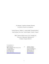
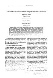
H. Quené, H. van den Bergh / Journal of Memory and Language 59 (2008) 413–425 419under H00 10 20 30 40F2(2,34)0 10 20 30 400 5 10 15 20under Ha+450 5 10 15 20F1(2,22)Fig. 1. Resulting F 1 and F 2 values of simulated data sets, with indication of significance of the fixed effect of condition, according tojoint F 1 and F 2 (open circles), minF 0 (filled circles), and crossed mixed-effects model (squares). Upper panel: without fixed effect ofcondition (according to H 0 ; 500 outcomes); lower panel: with fixed effect of condition (according to H a ; showing 455 of 500 outcomes).Dashed lines indicate critical F ratios.close to the nominal a = .05. These outcomes supportthe findings of Raaijmakers et al. (1999), who arguethat the current practice of reporting only F 1 and F 2is dangerous because it inflates the risk of a Type Ierror. The present simulations confirm this inflationof Type I error. Although many researchers regardminF 0 as too conservative for comfort, these simulationssuggest that it may even be too liberal, becauseit ignores the joint correlation within subjects andwithin items. This point is further addressed below.Application to response time dataIn order to further demonstrate the mixed-effectsmodeling with crossed random effects, we will analyzeresponse time data obtained from a phoneme monitor-

420 H. Quené, H. van den Bergh / Journal of Memory and Language 59 (2008) 413–425ing experiment. These response times were obtained in aDutch replication of the parallel English study by Quenéand Port (2005), which itself was a modification of asimilar study by Pitt and Samuel (1990). The 36 participantswere instructed to press a response button as soonas they heard a pre-specified target phoneme in a list ofspoken disyllabic words (Connine & Titone, 1996). Thecritical factor was whether the word list had regular timing(isochronous intervals between stressed syllables) orirregular timing (non-isochronous intervals); fasterresponses are predicted for the regularly timed stimulias compared to the irregular-timed stimuli. The stresspattern of the target word, being either trochaeic(strong–weak) or iambic (weak–strong), constituted asecond factor in this study. As a third factor, the targetphoneme occurred either in the first or in the secondsyllable.Hence, there are three fixed effects, viz. regularity(within items, within participants), stress pattern, andtarget position (both varying between-items, within-participants).For each of the four cells defined by the lattertwo factors, 24 target words were selected, with anappropriate target phoneme in the appropriate position.The 4 24 Dutch items were rotated over the presentationconditions, so that a participant heard a particulartarget words only once, yielding four different versionsof the experiment (with nine participants per version).Response times were measured from the onset of the targetphoneme. The individual responses were stored inunivariate format, i.e. each row of the data file correspondsto a single response, with participant, item, factorvalues (and additional information) coded in eachrow. RTs were transformed to their logarithmic values,in order to remove the intrinsic positive skew and nonnormalityof their distribution (Keene, 1995; Limpert,Stahel, & Abbt, 2001). There were 198 missing responses(6%); these were simply discarded and not imputed.As above, the preliminary mixed-effects model containsonly the intercept or ‘‘grand mean” in its fixed part.In the random part (in parentheses), the total variance isdecomposed into three components, viz. variancebetween participants r 2 u 0ðj0Þ, variance between test itemsr 2 v 0ð0kÞ, and residual variance nested under the combinationof participants and test items r 2 e iðjkÞ.logðY iðjkÞ Þ¼c 0ð00Þ þ u 0ðj0Þ þ v 0ð0kÞ þ e iðjkÞð10ÞThe estimated coefficients for this model are shown inTable 3. The variance between items r 2 v 0ð0kÞis considerablylarger than the variance between participantsr 2 u 0ðj0Þ, as expected, because two of the factors of interestvary between test items. Hence, the between-items variancein the empty model reflects systematic effects underinvestigation.The next step is to include the fixed factors of interestto the model. All three factors are binary (having twolevels), and they are entered as a single dummy factor,with value 1 or ‘‘on” indicating timing being regular(hence, TR), stress falling on the second syllable (i.e., atrochee target word, hence, S2), and the target phonemebeing positioned in the second syllable (hence, P2),respectively. Because of this parameterization of termsin the model, the main effect of timing regularity modelsthis effect in the condition with trochee target words(dummy for stress equals zero) with the target phonemein the first syllable (dummy for position equals zero).Relevant two-way interactions are also included. (Thetwo-way interaction between regularity and target positionwas never significant, and it has been eliminatedhere for clarity.) The estimated coefficients are also listedin Table 3. Note that the random variance between itemsis greatly reduced, now that a considerable part of thisvariation has been captured in the fixed part of theregression model. Each main effect is significant, becauseits t value (estimate divided by standard error) evenexceeds the critical value t :95¼ 2:03 for 36 df.Next, it should be verified whether the data areindeed homoscedastic, as assumed by this regressionmodel. This was done by including each main effect intothe random part at both the levels of participants and ofitems, and evaluating all these candidate models bymeans of their likelihood values, as outlined above.Based on this exploration, the optimal model containsthe effect of regularity both in the fixed part and in therandom part at the items level:log Y iðjkÞ ¼ c0ð00Þ þ c TR0ð00Þ TR þ c S2 0ð00Þ S2þ c P2 0ð00Þ P2 þ c TR:S2 0ð00Þ TRS2þ c S2:P2 0ð00Þ S2P2þ u 0ðj0Þ þ v 0ð0kÞ þ v TR 0ð0kÞ TR þ e iðjkÞð11ÞThe estimated coefficients in Table 3 for this finalmodel (11) show that the main effect of regularity isno longer significant, if this effect is also included inthe random part of the model. In other words, thebetween-items variability is considerably larger in theregular-timing condition than in the irregular-timingcondition. If this heteroschadasticity is taken intoaccount, then items with initial stress do not show a significanteffect of regularity any more (due to the largerstandard error of the estimate; t = 1.79). For itemswith final stress, however, the regularity effect is stillhighly significant (t = 3.81). As before, we see thatameliorating the random part, to account better for randomvariation, lowers the significance levels for the fixedeffects, thus reducing the risk of capitalization onchance.The results of this study involving lists of spokenwords confirm that regular speech rhythm facilitatesspoken-word perception, yielding faster reaction

Table 3Estimated parameters (with standard error of estimate in parentheses) of mixed-effects modeling of response times obtained in aphoneme monitoring experimentModel (10) Model (11)Fixedc 0ð00Þ 6.269 (0.037) 6.338 (0.036) 6.338 (0.038)c TR 0ð00Þ 0.040 (0.016) * 0.041 (0.023)c S2 0ð00Þ 0.275 (0.032) * 0.281 (0.036) *c P20ð00Þ 0.245 (0.031) * 0.245 (0.030) *c TR:S2 0ð00Þ 0.121 (0.023) * 0.121 (0.032) *c S2:P2 0ð00Þ 0.015 (0.043) 0.002 (0.042)Randomr 2 u 0ðj0Þ0.028 0.028 0.0279r 2 v 0ð0kÞ0.052 0.008 0.0149r 2 v TR 0ð0kÞ0.0121r 2 e iðjkÞ0.110 0.107 0.1035Evaluation2 log(lh) 2446 2188 2156v 2 deviance(1 df) 32p deviance

422 H. Quené, H. van den Bergh / Journal of Memory and Language 59 (2008) 413–4250.16, and 0.11. In logistic modeling, the hit rates are firstconverted to logit units [i.e. to the logarithm of the oddsof hits: logitðPÞ ¼logðP=ð1 PÞÞ], which are thenregressed onto the predictors in the model. Here therespective hit rates correspond to logit values of1.174, 1.660, and 2.044, respectively. Note thatnegative logit values correspond to hit rates below .5.As before, we start by fitting the empty model.Instead of aggregating over participants, or over items,however, we model the raw hits themselves. This meansthat we can also specify a model with crossed randomfactors, i.e., the logistic equivalent of model (8):logit Y iðjkÞ¼ c0ð00Þ þ u 0ðj0Þ þ v 0ð0kÞð12ÞBecause of the computational complexities outlinedabove, it is not possible to estimate variance componentsfor residuals, as these are implied by the mean(s). Becausewe have specified crossed random factors, the intra-groupcorrelation cannot be reported. The resultingestimates are listed in Table 4.The subsequent model has the condition effect in itsfixed part only. The difference with conventional RM-ANOVA is that both participants and items are againincluded as two crossed random factors:logit Y iðjkÞ¼ cH0ð00Þ H þ c N0ð00Þ N þ c L0ð00Þ Lþ u 0ðj0Þ þ v 0ð0kÞð13ÞThe joint contrasts among the dummies’ coefficients inthe fixed part yield a significant main effect: v 2 = 14.96,p < .001, which suggests significant differences in hitrates among the three conditions. The conventionalRM-ANOVA reports a (marginally) significant main effectin both analyses [F 1 (2,22) = 3.2, p = .058;F 2 (2,34) = 6.3, p = .005] although the minF 0 value isnot significant [minF 0 (2,43) = 2.13, p = .131].As before, we verify whether the assumption ofhomoscedasticity is warranted, by evaluating candidatemodels having the predictors in the random part. Thisshows that the between-subject variance r 2 u 0ðj0Þvariesamong the treatment conditions, much like the originalcontinuous variable did (cf. Model (9)):logit Y iðjkÞ¼ cH0ð00Þ H þ c N0ð00Þ N þ c L0ð00Þ Lþ u H0ðj0Þ H þ u N0ðj0Þ N þ u L0ðj0Þ L þ v 0ð0kÞð14ÞThe estimated coefficients for this final model are alsolisted in Table 4. The far larger variance between participantsin the Low condition is now represented correctly inthe random part, and not in the fixed part. This results in alarger standard error (less confidence) in the estimate forthis condition in the fixed part, which in turn results inthe main effect being not significant [v 2 (2) = 4.39,p = .111]. As before, an artefactually significant effect inthe fixed part (i.e., a Type I error) has disappeared whenthe random part was ameliorated. Although the two models(13) and (14) perform equally well [as indicated by theirnon-significant deviance, v 2 (2) = 3.3, p = .192], we preferthe latter model, because it better captures the lower confidencefor very low (or very high) hit rates.Discussion and conclusionThe exposition above has demonstrated that mixedeffectsmodeling provides an excellent tool for analyzingTable 4Estimated parameters (with standard error of estimate in parentheses) of mixed-effects modeling of fictitious binomial data (see text fordetails)Model (12) Model (13) Model (14)Fixedc 000 1.585 (0.256)c H000 1.174 (0.279) 1.174 (0.260)c N000 1.660 (0.290) 1.660 (0.273)c L000 2.045 (0.304) 2.045 (0.405)Randomr 2 u 0ðj0Þ0.943 (0.332) 0.968 (0.340)r 2 u H0ðj0Þ0.830 (0.380)r 2 u N0ðj0Þ0.715 (0.393)r 2 u L0ðj0Þ2.807 (1.055)r 2 v 0ð0kÞ0.642 (0.223) 0.653 (0.227) 0.612 (0.219)Evaluation2 log(lh) 652.7 611.7 615.0v 2 deviance(2 df) 3.3p deviance .192v 2 condition(2 df) n/a 14.96 4.39p condition

H. Quené, H. van den Bergh / Journal of Memory and Language 59 (2008) 413–425 423data from psycholinguistic experiments. Multiple randomfactors can be included into a single analysis, whichessentially solves the ‘‘language-as-fixed-effect-fallacy”that has plagued researchers for decades (Clark, 1973;Meuffels & van den Bergh, 2006). The multiple randomfactors can be nested (e.g. observations within participants,for repeated-measures designs with independentobservations across participants), or they can be crossed(e.g. items and participants, for repeated-measuresdesigns where observations are also correlated acrossparticipants). Well-established techniques are availablefor modeling data that are normally distributed (perhapsafter some data transformation, as illustrated above)and for binomial data. Models for other distributionare also under current development.Only a few years ago, mixed-effects modeling was acomplicated operation requiring specialized software,which often imposed a steep learning curve. So far thishas prevented mixed-effects modeling from becomingstandard routine in behavioral linguistic research, contraryto other disciplines. Since powerful and convenientimplementations have now become available, however,running one mixed-effects model is often easier than runningtwo RM-ANOVAs. Hence, there is little reason tomaintain the conventional RM-ANOVA routine ofcomputing and combining F 1 and F 2 .The results above also indicate that mixed-effects modelsare typically more conservative than conventionalRM-ANOVA, at least for designs with crossed randomeffects. In our Monte Carlo simulations above, the powerof the fixed effect of condition was .90 for analyses usingminF 0 , and .89 for crossed mixed-effects analyses. In otherstudies the reduction of power may not be so mild,depending on the actual experimental design, and thedegrees of heteroscedasticity, of asphericity, and ofintra-group correlation (cf. Kreft & De Leeuw, 1998,chap. 5.4). [For nested designs, however, multilevel analysisseems to be more powerful than a single RM-ANOVA, Quené and van den Bergh (2004)]. The conservativebehavior of crossed mixed-effects models is neverthelessappropriate, as the following metaphorillustrates. Let us regard the data set under analysis as asponge, soaked with information. The water in the spongerepresents the variance in the data set. Our researchhypothesis is concerned with the true variance (water)related to the fixed effects in our study. Hence, we haveto squeeze out of the sponge as much of the random varianceas we can, leaving only the fixed variance within thesponge, and we catch that squeezed-out random variancein a bucket. In RM-ANOVA, we are limited to use onlyone hand for squeezing. So, we squeeze with the righthand (yielding F 1 ), we take an exact copy of the soakedsponge, and we squeeze that with the left hand (yieldingF 2 ). In both squeezes, however, some amount of randomvariance (water) is inadvertedly left in the sponge, becausesqueezing can only be done imperfectly with a single hand.In both analyses, this remaining random variance weighsin with the fixed-effect variance in the sponge, instead ofwith the random variance in the bucket. Hence, to mixmetaphors, it inflates the significance of the fixed effect,and may result in a false positive outcome, or Type I error.In mixed-effects modeling, by contrast, we use both handsfor squeezing. This allows us to squeeze more random variance(water) out of the sponge. After squeezing, theamount of variance (water) within the sponge is smaller,and the amount in the bucket is larger, because of ourmore effective two-handed squeezing. Because theamount of random variance (water) that is left in thesponge instead of the bucket is now smaller, the evaluationof the fixed effects will be better. The less liberalbehavior of mixed-effects analysis, relative to minF 0 analyses,provides a better protection against capitalization onchance.If the language items under study (e.g. target words)are regarded as a random sample from a larger populationof these items, i.e. as a random effect, then crossed mixedeffectsmodels effectively solve the ‘‘language-as-fixedeffects-fallacy”,as argued before. However, includingitems as a random effect in a crossed mixed-effects modeldoes not in itself provide information about the generalityof the fixed effect(s) over these items (as noted by LeonardKatz in the internet-based debate about F 2 ; see Forster,this issue, for an introduction). Such a measure of generalitywould even go against this model, precisely becauseitems are assumed to be randomly selected, and hence,as essentially homogeneous in their susceptibility to thefixed effect. Moreover, an interaction of items by treatmentscannot be evaluated in an incomplete design suchas the latin-square designs discussed here. Unless all combinationsof subjects and items are tested under all treatmentconditions, the two-way interactions of items bytreatments and of subjects by treatments are confoundedwith the main effect of treatment (Bailey, 1982; Cox, 1958;Janse & Quené, 2004). What analysts can do, however, isinspect and compare the residuals of the items (cf. Afshartous& Wolf, 2007), and attempt to relate these to somerelevant property of the items. This property (e.g. partof speech, lexical frequency, etc.) may then be includedas a tentative fixed between-item predictor in their candidatemodels, and it may be tested for its main effect and forinteractions with the fixed treatment effects under study.In an educational analogy, we can evaluate the fixed effectof treatment on students’ performance, but we cannotevaluate the interaction of treatment and students, if studentswere indeed sampled at random. Relevant propertiesof the students, e.g. IQ score, may however be usedas additional fixed predictors of the treatment effect, andof the variation in students’ individual intercepts and instudents’ slopes of the treatment effect.Mixed-effects modeling thus offers considerableadvantages over RM-ANOVA techniques, as discussedabove. This technique also allows researchers to com-

424 H. Quené, H. van den Bergh / Journal of Memory and Language 59 (2008) 413–425bine discrete and categorical predictors into a singlemodel, it does not require homoscedasticity nor sphericity,it does not require aggregation of binomial data, andit is robust against missing data. In conclusion, mixedeffectsmodeling provides a superior means of statisticalanalyses in our discipline, and adopting this technique ishighly recommended to improve our research into languageand speech behavior.AcknowledgmentsHugo Quené and Huub van den Bergh, Utrecht instituteof Linguistics OTS, Utrecht University.Our thanks are due to Douglas Bates for technicalassistance, to Esther Janse and Sieb Nooteboom forhelpful discussions, and to Tom Lentz, Harald Baayenand two anonymous reviewers for valuable commentsand suggestions.ReferencesAfshartous, D., & Wolf, M. (2007). Avoiding ‘data snooping’ inmultilevel and mixed effects models. Journal of the RoyalStatistical Society Series A (Statistics in Society), 170(4),1035–1059.Baayen, R. H., Davidson, D. J., & Bates, D. M. (2008). Mixedeffects modeling with crossed random effects for subjectsand items. Journal of Memory and Language, 59, 390–412.Baayen, R. H., Tweedie, F. J., & Schreuder, R. (2002). Thesubjects as a simple random effect fallacy: Subject variabilityand morphological family effects in the mental lexicon.Brain and Language, 81(1–3), 55–65.Bailey, R. (1982). Confounding. In N. Johnson & S. Kotz(Eds.). Encyclopedia of statistical sciences (Vol. 2,pp. 128–134). New York: Wiley.Bates, D. (2005). Fitting linear models in R: Using the lme4package. R News, 5(1), 27–30.Clark, H. (1973). The language-as-fixed-effect fallacy: A critiqueof language statistics in psychological research. Journal ofVerbal Learning and Verbal Behavior, 12, 335–359.Cnaan, A., Laird, N. M., & Slasor, P. (1997). Using the generallinear mixed model to analyse unbalanced repeated measuresand longitudinal data. Statistics in Medicine, 16(20),2349–2380.Cochran, W., & Cox, G. (1957). Experimental designs. NewYork: Wiley.Connine, C. M., & Titone, D. (1996). Phoneme monitoring.Language and Cognitive Processes, 11(6), 635–645.Cox, D. (1958). Planning of experiments. New York: Wiley.Faraway, J. J. (2006). Extending the linear model with R:Generalized linear, mixed effects and nonparametric regressionmodels. Boca Raton, FL: Chapman and Hall.Goldstein, H. (1999). Multilevel statistical models (2nd (electronicupdate) ed.). London: Edward Arnold.Guo, G., & Zhao, H. (2000). Multilevel modeling for binarydata. Annual Review of Sociology, 26, 441–462.Hoffmann, L., & Rovine, M. J. (2007). Multilevel models forthe experimental psychologist: Foundations and illustrativeexamples. Behavior Research Methods, 39(1), 101–117.Hosmer, D. W., & Lemeshow, S. (2000). Applied logisticregression (2nd ed.). New York: Wiley.Hox, J. (1995). Applied multilevel analysis. Amsterdam: TTPublicaties.Janse, E., & Quené, H. (2004). On measuring multiple lexicalactivation using the cross-modal semantic priming technique.In H. Quené & V. J. van Heuven (Eds.), On speechand language: Studies for Sieb G. Nooteboom (pp. 105–114).Utrecht: LOT.Keene, O. N. (1995). The log transformation is special.Statistics in Medicine, 14, 811–819.Kleinbaum, D. G. (1992). Logistic regression: A self-learningtext. New York: Springer.Kreft, I. G., & De Leeuw, J. (1998). Introducing multilevelmodeling. London: Sage.Limpert, E., Stahel, W. A., & Abbt, M. (2001). Lognormaldistributions across the sciences: Keys and clues. Bioscience,51(5), 341–352.Luke, D. A. (2004). Multilevel modeling. Thousand Oaks, CA:Sage.Maxwell, S. E., & Delaney, H. D. (2004). Designing experimentsand analyzing data: A model comparison perspective (2nded.). Mahwah, NJ: Lawrence Erlbaum Associates.Meuffels, B., & van den Bergh, H. (2006). De ene tekst is deandere niet: The language-as-fixed-effect fallacy revisited:Statistische implicaties. Tijdschrift voor Taalbeheersing,28(4), 323–345.O’Brien, R. G., & Kaiser, M. K. (1985). MANOVA method foranalyzing repeated measures designs: An extensive primer.Psychological Bulletin, 97(2), 316–333.Pampel, F. C. (2000). Logistic regression: A primer. ThousandOaks, CA: Sage.Pinheiro, J. C., & Bates, D. M. (2000). Mixed-effects models in Sand S-Plus. New York: Springer.Pitt, M. A., & Samuel, A. G. (1990). The use of rhythm inattending to speech. Journal of Experimental Psychology:Human Perception and Performance, 16(3), 564–573.Pollatsek, A., & Well, A. D. (1995). On the use of counterbalanceddesigns in cognitive research: A suggestion for abetter and more powerful analysis. Journal of ExperimentalPsychology: Learning, Memory, and Cognition, 21(3),785–794.Quené, H. (2008). Multilevel modeling of between-speaker andwithin-speaker variation in spontaneous speech tempo.Journal of the Acoustical Society of America, 123(2),1104–1113.Quené, H., & Port, R. (2005). Effects of timing regularity andmetrical expectancy on spoken-word perception. Phonetica,62(1), 1–13.Quené, H., & van den Bergh, H. (2004). On multi-levelmodeling of data from repeated measures designs: Atutorial. Speech Communication, 43(1–2), 103–121.R Development Core Team. (2008). R: A language andenvironment for statistical computing. R Foundation forStatistical Computing. [Computer program (version 2.6.2)].Available from: http://www.r-project.org.Raaijmakers, J. G., Schrijnemakers, J. M., & Gremmen, F.(1999). How to deal with ‘‘the language-as-fixed-effect

H. Quené, H. van den Bergh / Journal of Memory and Language 59 (2008) 413–425 425fallacy”: Common misconceptions and alternative solutions.Journal of Memory and Language, 41, 416–426.Rasbash, J., Browne, W., Goldstein, H., Yang, M., Plewis, I.,Healy, M., et al. (2000). A user’s guide to MLwiN(Computer program (version 2.02) and manual. Availablefrom: http://www.cmm.bristol.ac.uk/team/userman.pdf).Multilevel Models Project, Institute of Education, Universityof London.Raudenbush, S. W., & Bryk, A. S. (2002). Hierarchical linearmodels: Applications and data analysis methods (2nd ed.).Thousand Oaks, CA: Sage.Richter, T. (2006). What is wrong with ANOVA andmultiple regression? Analyzing sentence reading timeswith hierarchical linear models. Discourse Processes,41(3), 221–250.Rietveld, T., & Van Hout, R. (2005). Statistics in languageresearch: Analysis of variance. Berlin: Mouton de Gruyter.Searle, S. R., Casella, G., & McCulloch, C. E. (1992). Variancecomponents. New York: Wiley.Snijders, T., & Bosker, R. (1999). Multilevel analysis: Anintroduction to basic and advanced multilevel modeling.London: Sage.van der Leeden, R. (1998). Multilevel analysis of repeatedmeasures data. Quality and Quantity, 32, 15–19.Winer, B. (1971). Statistical principles in experimental design(2nd ed.). New York: McGraw-Hill.