EconS 491: Strategy and Game Theory Oligopoly games with ...

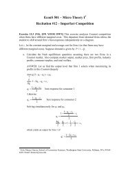
Firm 1. Let us now analyze Firm 1 (the uninformed player in this game). First note that its
pro…ts must be expressed in expected terms, since …rm 1 does not know whether …rm 2 has low or
high costs.
Rearranging,
1
P rofits 1 =
2
P rofits 1 = 1 2 (1 q 1 q2 L )q 1
| {z }
if low costs
q 1
2
q L 2
2 + 1 2
q 1
2
q H 2
2
+ 1 2 (1 q 1 q H 2 )q 1
| {z }
if high costs
q2
L q 1 = 1 q 1
2
q H 2
2
q 1
= q 1 (q 1 ) 2 q L 2
2 q 1
q H 2
2 q 1
Di¤erentiating with respect to q 1 , we can obtain …rm 1’s best response function, BRF 1 (q L 2 ; qH 2 ):
Note that we do not have to di¤erentiate for the case of low and high costs, since …rm 1 does not
observe such information). In particular,
1 2q 1
q L 2
2
q2
H 2 = 0 =) q 1 q2 L ; q2
H 1 =
2
q L 2
2
q H 2
2
(BRF 1 (q L 2 ; qH 2 ))
After …nding the best response functions for both types of Firm 2 and for the unique type of
Firm 1 we are ready to plug the …rst two BRFs into the latter. Speci…cally,
q 1 = 1 2
1 q 1
2
2
3
8
2
q 12
And solving for q 1 , we …nd q 1 = 3 8 .
With this information, it is easy to …nd the particular level of production for …rm 2 when
experiencing low marginal costs,
q L 2 (q 1 ) = 1 q 1
2
= 1 3
8
2
= 5
16
As well as the level of production for …rm 2 when experiencing high marginal costs,
q H 2 (q 1 ) = 3 8
3
8
2 = 3
16
Therefore, the Bayesian Nash equilibrium of this oligopoly game with incomplete information
about …rm 2’s marginal costs prescribes the following production levels
q 1 ; q L 2 ; q H 2
=
3
8 ; 5 16 ; 3 16
2