EconS 491: Strategy and Game Theory Oligopoly games with ...

EconS 424: Strategy and Game Theory
Oligopoly games with incomplete information
about …rms’cost structure
March 7, 2014
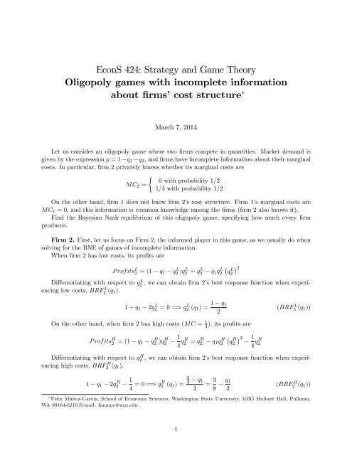
Let us consider an oligopoly game where two …rms compete in quantities. Market demand is
given by the expression p = 1 q 1 q 2 , and …rms have incomplete information about their marginal
costs. In particular, …rm 2 privately knows whether its marginal costs are
0 with probability 1/2
MC 2 =
1=4 with probability 1/2
On the other hand, …rm 1 does not know …rm 2’s cost structure. Firm 1’s marginal costs are
MC 1 = 0, and this information is common knowledge among the …rms (…rm 2 also knows it).
Find the Bayesian Nash equilibrium of this oligopoly game, specifying how much every …rm
produces.
Firm 2. First, let us focus on Firm 2, the informed player in this game, as we usually do when
solving for the BNE of games of incomplete information.
When …rm 2 has low costs, its pro…ts are
P rofits L 2 = (1 q 1 q2 L )q2 L = q2 L q 1 q2 L q2
L 2
Di¤erentiating with respect to q2 L , we can obtain …rm 2’s best response function when experiencing
low costs, BRF2 L(q 1).
1 q 1 2q L 2 = 0 =) q L 2 (q 1 ) = 1 q 1
2
(BRF L 2 (q 1))
On the other hand, when …rm 2 has high costs (MC = 1 4
), its pro…ts are
P rofits H 2 = (1 q 1 q H 2 )q H 2
1
4 qH 2 = q2 H q 1 q2 H q2
H 2 1
4 qH 2
, we can obtain …rm 2’s best response function when experi-
Di¤erentiating with respect to q2 H
encing high costs, BRF2 H(q 1).
1 q 1 2q H 2
1
4 = 0 =) qH 2 (q 1 ) =
3
4
q 1
2
= 3 8
q 1
2
(BRF H 2 (q 1))
Félix Muñoz-García, School of Economic Sciences, Washington State University, 103G Hulbert Hall, Pullman,
WA 99164-6210.E-mail: fmunoz@wsu.edu.
1

Firm 1. Let us now analyze Firm 1 (the uninformed player in this game). First note that its
pro…ts must be expressed in expected terms, since …rm 1 does not know whether …rm 2 has low or
high costs.
Rearranging,
1
P rofits 1 =
2
P rofits 1 = 1 2 (1 q 1 q2 L )q 1
| {z }
if low costs
q 1
2
q L 2
2 + 1 2
q 1
2
q H 2
2
+ 1 2 (1 q 1 q H 2 )q 1
| {z }
if high costs
q2
L q 1 = 1 q 1
2
q H 2
2
q 1
= q 1 (q 1 ) 2 q L 2
2 q 1
q H 2
2 q 1
Di¤erentiating with respect to q 1 , we can obtain …rm 1’s best response function, BRF 1 (q L 2 ; qH 2 ):
Note that we do not have to di¤erentiate for the case of low and high costs, since …rm 1 does not
observe such information). In particular,
1 2q 1
q L 2
2
q2
H 2 = 0 =) q 1 q2 L ; q2
H 1 =
2
q L 2
2
q H 2
2
(BRF 1 (q L 2 ; qH 2 ))
After …nding the best response functions for both types of Firm 2 and for the unique type of
Firm 1 we are ready to plug the …rst two BRFs into the latter. Speci…cally,
q 1 = 1 2
1 q 1
2
2
3
8
2
q 12
And solving for q 1 , we …nd q 1 = 3 8 .
With this information, it is easy to …nd the particular level of production for …rm 2 when
experiencing low marginal costs,
q L 2 (q 1 ) = 1 q 1
2
= 1 3
8
2
= 5
16
As well as the level of production for …rm 2 when experiencing high marginal costs,
q H 2 (q 1 ) = 3 8
3
8
2 = 3
16
Therefore, the Bayesian Nash equilibrium of this oligopoly game with incomplete information
about …rm 2’s marginal costs prescribes the following production levels
q 1 ; q L 2 ; q H 2
=
3
8 ; 5 16 ; 3 16
2

EconS 424: Strategy and Game Theory
Oligopoly games with incomplete information
about market demand
March 7, 2014
Let us consider an oligopoly game where two …rms compete in quantities. Both …rms have the
same marginal costs, MC = $1, but they are asymmetrically informed about the actual state of
market demand. In particular, Firm 2 does not know what is the actual state of demand, but
knows that it is distributed with the following probability distribution
10 Q with probability 1/2
p(Q) =
5 Q with probability 1/2
On the other hand, …rm 1 knows the actual state of market demand, and …rm 2 knows that
…rm 1 knows this information (i.e., it is common knowledge among the players).
Firm 1. First, let us focus on Firm 1, the informed player in this game, as we usually do when
solving for the BNE of games of incomplete information.
When …rm 1 observes a high demand market its pro…ts are
P rofits 1 = (10 Q)q H 1 1q H 1
= (10 q H 1 q 2 )q H 1 q H 1
= 10q H 1 q H 1
2
q 2 q H 1 1q H 1
, we can obtain …rm 1’s best response function when experi-
Di¤erentiating with respect to q1 H
encing low costs, BRF1 H(q 2).
10 2q H 1 q 2 1 = 0 =) q H 1 (q 2 ) = 4:5
On the other hand, when …rm 1 observes a low demand market its pro…ts are
q 2
2
(BRF H 1 (q 2))
P rofits 1 = (5 q L 1 q 2 )q L 1 1q L 1 = 5q L 1 q L 1
2
q 2 q L 1 1q L 1
Di¤erentiating with respect to q1 L , we can obtain …rm 1’s best response function when experiencing
high costs, BRF1 L(q 2).
5 2q L 1 q 2 1 = 0 =) q L 1 (q 2 ) = 2
q 2
2
(BRF L 1 (q 2))
Félix Muñoz-García, School of Economic Sciences, Washington State University, 103G Hulbert Hall, Pullman,
WA 99164-6210.E-mail: fmunoz@wsu.edu.
1

Firm 2. Let us now analyze Firm 2 (the uninformed player in this game). First note that its
pro…ts must be expressed in expected terms, since …rm 2 does not know whether market demand
is high or low.
Rearranging,
P rofits 2 = 1
(10 q
H
2 1 q 2 )q 2 1q 2 + 1
(5 q
L
| {z } 2 1 q 2 )q 2 1q 2
| {z }
demand is high
demand is low
P rofits 2 = 1 2
i
h10q 2 q1 H q 2 (q 2 ) 2 q 2 + 1 i
h5q 2 q1 L q 2 (q 2 ) 2 q 2
2
Di¤erentiating with respect to q 2 , we can obtain …rm 2’s best response function, BRF 2 (q L 1 ; qH 1 ):
Note that we do not have to di¤erentiate for the case of low and high demand, since …rm 2 does
not observe such information). In particular,
Rearraging,
And solving for q 2 ,
q 2 q L 1 ; q H 1
1
10 q
H
2 1 2q 2 1 + 1
5 q
L
2 1 2q 2 1 = 0
=
13 q L 1 q H 1
4
13 q H 1 4q 2 q L 1 = 0
= 3:25 0:25 q1 L + q1
H
(BRF 2 q1 L; qH 1 )
After …nding the best response functions for both types of Firm 1 and for the unique type of
Firm 2 we are ready to plug the …rst two BRFs into the latter. Speci…cally,
0
1
h
q 2 = 3:25 0:25 B 2
@
And solving for q 2 , we …nd q 2 = 2:167.
q 2
i
| {z 2 }
q1
L
h
+
i
C
2 A
q 2
4:5
| {z }
q1
H
With this information, it is easy to …nd the particular level of production for …rm 1 when
experiencing low market demand,
q L 1 (q 2 ) = 2
q 2
2 = 2 2:167
= 0:916
2
As well as the level of production for …rm 1 when experiencing high market demand,
q H 1 (q 2 ) = 4:5
q 2
2 = 4:5 2:167
= 3:4167
2
Therefore, the Bayesian Nash equilibrium (BNE) of this oligopoly game with incomplete
information about market demand prescribes the following production levels
q H 1 ; q L 1 ; q 2
= (3:416; 0:916; 2:167)
2