Numerical solutions of magnetohydrodynamic equations - Lublin

BULLETIN OF THE POLISH ACADEMY OF SCIENCES
TECHNICAL SCIENCES, Vol. 59, No. 1, 2011
DOI:
Numerical solutions of magnetohydrodynamic equations
K. MURAWSKI ∗
Faculty of Mathematics, Physics and Informatics, UMCS, 10 Radziszewskiego St., 20-031 Lublin, Poland
Abstract. In this paper we review several mathematical aspects in numerical methods for magnetohydrodynamic equations. The intrinsic
complexity and the requirements of the selenoidity condition make numerical solutions of these equations a formidable task. We present
results of advanced numerical simulations for a complex system, which reveal that the numerical methods cope very well with this task.
Key words: numerical methods for hyperbolic equations, finite volume methods, Godunov-type methods, magnetohydrodynamics.
1. Introduction
The magnetohydrodynamic (MHD) theory is the simplest selfconsistent
model describing the macroscopic behavior of the
plasma. Despite of that the full nonlinear equations are so
complex that usually significant simplifications are necessary
to yield analytically tractable problems. As a result, the MHD
equations usually require numerical treatment. Finite-volume
methods [1] are one of several different techniques available to
solve the MHD equations. They are simple to implement, easily
adaptable to complex geometries, and well suited to handle
nonlinear terms. Like solutions of nonlinear equations, perturbations
described by the MHD equations may result in large
gradients which are difficult for numerical modeling. The use
of standard numerical schemes of second-order accuracy or
higher (e.g., the Lax-Fredrichs method) generates spurious
oscillations which destroy monotonicity of the solution [2].
Lower-order schemes [3] are generally free of oscillations,
but they are too dissipative [1]. Therefore, a development of
more advanced schemes, which could adequately represent
the large gradient profiles, was required.
Due to the intrinsic complexity of the MHD equations,
the development of numerical techniques to solve these equations
was slower than for hydrodynamics (HD). For a long
time most numerical schemes were based on methods dependent
on artificial viscosity to represent adequately shocks [4].
Although these schemes were successfully applied in the
past [5], recent experience with fully conservative, high-order
upwind hydrodynamic codes found latter to be superior in
many applications [6]. It is therefore natural to extend such
schemes to solve the MHD equations. However, converting
a HD code to a MHD code is a difficult task. The difficulty
results from the fact that the MHD equations possess new
families of waves such as switch-on fast shocks, switch-off fast
rarefactions, switch-off slow shocks, and switch-on slow rarefactions
[7, 8]. It is also possible to obtain compound waves
of either fast or slow waves. This exerts a considerable impact
on a performance of the algorithms which are required to
provide accurate capture of the entire range of such structures
[9]. The other difficulty is that the MHD equations contain
the magnetic field which has to satisfy the divergence-free
constraint. A local nonzero divergence of magnetic field indicates
the existence of magnetic monopoles within the numerical
cell, which leads to non-conservation of the magnetic flux
across its surface. Accumulation of the numerical errors associated
with evolving the magnetic field components can lead
to violation of this constraint, causing an artificial force parallel
to the magnetic field, and eventually can force termination
of the simulations.
Despite of the above reported problems many numerical
schemes were developed for the MHD equations. These
schemes reveal either conservative or non-conservative properties
of the equations. The aim of this paper is to review some
recently devised numerical methods for solving the MHD
equations, which are illustrated in Sec. 2. Some problems
present in numerical schemes for the MHD equations are discussed
in Sec. 3. Results of numerical simulations of impulsively
generated waves in a strongly stratified atmosphere are
presented in Sec. 4. This paper is completed by summary of
the main results.
2. MHD equations
The MHD equations can be written in the following form:
∂̺
+ ∇ · (̺V) = 0,
∂t
(1)
̺∂V
∂t + ̺ (V · ∇)V = −∇p + 1 (∇ × B) × B + ̺g, (2)
µ
∂B
= ∇ × (V × B),
∂t
(3)
∇ · B = 0, (4)
∂p
+ ∇ · (pV) = (1 − γ)p∇ · V,
∂t
(5)
p = k B ̺T. (6)
m
Here ̺ is mass density, V is flow velocity, B is the magnetic
field, p is gas pressure, γ = 5/3 is the adiabatic index,
g is gravitational acceleration, T is temperature, m is mean
particle mass and k B is the Boltzmann’s constant.
∗ e-mail: kmur@kft.umcs.lublin.pl
1

K. Murawski
is the pressure scale-height, and p 0 denotes the gas pressure
at the reference level, y = y r , which we choose and set fixed
as y r = 10 Mm.
We adopt a realistic temperature profile T(y) for the solar
atmosphere [30], which is displayed in Fig. 1. Note that T
attains a value of about 5700 K at the top of the photosphere
which corresponds to y = 0.5 Mm. At higher altitudes T(y)
falls off until it reaches its minimum of 4350 K at the altitude
of y ≃ 0.95 Mm. Higher up T(y) grows gradually with height
up to the transition region which is located at y ≃ 2.7 Mm.
Here T(y) experiences a sudden growth up to the coronal
value of 1.5 MK at y = 10 Mm. Having specified T(y) with
a use of Eqs. (55) and (60) we can obtain mass density and
gas pressure profiles.
Fig. 1. Equilibrium temperature (in Kelvins) profile vs. height y (in
Mm) for the solar atmosphere
For the initial magnetic field, we adopt the model which
was devised by Priest [31]. In this model, we assume that
magnetic field is current-free (∇ × B = 0) and potential
(B = ∇ × (Aẑ)) with the magnetic flux function
A(x, y) = B 0 Λ B cos(x/Λ B )exp[−(y − y r )/Λ B ] . (58)
Here B 0 denotes the magnetic field at y = y r and Λ B = 2L/π
is the magnetic scale-height. We choose 2L = 30 Mm which
correspond to the size of a supergranular cell. It is noteworthy
that the magnetic field is predominantly vertical at supergranular
boundaries (x = 0, x = 2L), while it reveals a horizontal
canopy structure at the supergranular center (x = L).
A magnitude of magnetic field is chosen to specify at
y = y r the plasma β = 2µp/B 2 = 2c 2 s /(γc2 A ) equal to 0.048.
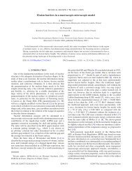
Here the sound speed c s = √ γp/̺ and the Alfvén speed,
c A = √ B 2 /(µ̺). Figure 2 illustrates vertical profile of the
plasma β which attains a value of about 0.015 around the
transition region, y ≃ 2.7 Mm, while it grows with depth
reaching a value of about 6 at y = 1.5 Mm that is located
within the solar chromosphere. This growth results from the
abrupt increase of gas pressure there.
Fig. 2. The plasma β profile vs. height y
We excite waves in the above described solar atmosphere
by launching initially, at t = 0, the Gaussian pulse in a vertical
component of velocity V y , i.e.
V y (x, y, t = 0) = A v exp
[− x2 + (y − y 0 ) 2 ]
w 2 . (59)
Here A v = 5 km s −1 is the amplitude of the pulse, y 0 =
0.5 Mm is its vertical position and w = 0.3 Mm is its width.
Equations (1)–(6) are solved numerically using the code
FLASH [27] which implements a second-order unsplit Godunov
solver and Adaptive Mesh Refinement (AMR). We set
the simulation box as (−15, 15) Mm ×(−0.5, 29.5) Mm and
fix at all four boundaries of the simulation region the plasma
quantities to their equilibrium values. In our studies we use
AMR grid with a minimum (maximum) level of refinement
blocks set to 5 (8). The refinement strategy is based on controlling
numerical errors in a gradient of mass density. Such
settings result in an excellent resolution of steep spatial profiles,
which significantly reduce numerical diffusion within
the simulation region.
Figure 3 illustrates spatial profiles of log̺ and velocity
vectors at t = 250 s (left panel) and t = 1500 s (right
panel). The initial pulse splits in a usual way into counterpropagating
waves. The wave propagating upwards grows in
its amplitude as a result of the rapid decrease of mass density
in the chromosphere. As a consequence of that a shock
results in. Photospheric and chromospheric plasma is lifted
up by underpressure which settles in below the shock. The
pressure gradient force overwhelms gravity and it pushes the
photospheric and chromospheric material towards the solar
corona. This scenario is clearly seen at t = 250 s. At a later
time the plasma becomes attracted by gravity and as a result is
falls off towards the low layers. However, the secondary shock
which results from the original pulse works against this fall off
as it lifts up the photospheric and chromospheric plasma. As
a result, a complex bi-directional flows arises. The whole scenario
bares many features of solar spicules. It is noteworthy
that the magnetic field-free case, B = 0, was recently discussed
by Gruszecki et al. [32] who revealed similar features
of quasi-periodic shocks traveling from the chromosphere to
the corona. However, in this hydrodynamic case spatial wave
profiles were more symmetric in space and spicules were not
observed.
6 Bull. Pol. Ac.: Tech. 59(1) 2011

Numerical solutions of magnetohydrodynamic equations
Fig. 3. Mass density (colour maps, log scale) and velocity (arrows) profiles at t = 250 s (left panel) and t = 1500 s (right panel). Mass
density and velocity are expressed in units of 10 −12 kg m −3 and 1 Mm s −1 , respectively
Figure 4 displays time-signatures of the vertical component
of velocity for the case of Fig. 3. This velocity is collected
in time at the detection point (x = 0, y = 20) Mm.
The arrival of the shock front to the detection point occurs at
t ≃ 200 s. The second, third, and fourth shocks fronts reach
the detection point at t ≃ 350 s, t ≃ 650 s, and t ≃ 950 s,
respectively. This secondary shock results from the nonlinear
wake which lags behind the leading signal. In the linear approximation
and magnetic-free case, the wake oscillates with
the acoustic cut-off frequency
Ω ac = c s
2Λ
√
1 + 2 dΛ
dy . (60)
Fig. 4. The plasma β profile vs. height y
This scenario consists the building block of onedimensional
(1D) rebound shock model of [33] who proposed
that the secondary shock (or rebound shock) lifts up the transition
region higher than the first shock thereby resulting in
a spicule appearance at observed heights. The process is well
studied in the frame of 1D numerical simulations. However,
our 2D numerical simulations introduce new interesting
features in comparison to the 1D rebound shock scenario.
There are few conclusions which result from our simulations:
a) according to the theory of Klein-Gordon equation an initial
pulse generates a wave front and a trailing wake which
oscillates with acoustic cut-off frequency [33];
b) even a small amplitude initial pulse launched at the top
of the photosphere exhibits a tendency to generate shocks.
These shocks result from a nonlinear wake.
5. Summary
This paper presents several mathematical aspects in numerical
methods for magnetohydrodynamic equations. Although
this presentation is far from complete the emphasis is on the
methods which are the most effective and the best known to
the author.
There are several conditions that numerical schemes
should satisfy: accuracy and speed of numerical simulations,
adequate representation of complex flows and steep profiles,
lack of generation of spurious oscillations as well as robustness.
A computer code is called robust if it has the virtue of
giving reliable results to a wide range of problems without
needing to be retuned. Numerical schemes such as shockcapturing
schemes described in this paper satisfy these conditions.
Bull. Pol. Ac.: Tech. 59(1) 2011 7

K. Murawski
Existing numerical models such as was used in Sec. 4
with an adaptation of the FLASH code demonstrate the feasibility
of fluid simulations in obtaining at least qualitative and,
to some extent, quantitative features in the magnetized fluid.
With continued improvements in computational methods
and computer resources, the usefulness and capability of the
numerical approach should continue to improve.
Acknowledgements. The software used in this work was in
part developed by the DOE-supported ASCI/Alliance Center
for Astrophysical Thermonuclear Flashes at the University of
Chicago.
REFERENCES
[1] E. Toro, Riemann Solvers and Numerical Methods for Fluid
Dynamics, Springer, Berlin, 2009.
[2] R.J. LeVeque, Finite-volume Methods for Hyperbolic Problems,
Cambridge University Press, Cambridge, 2002.
[3] S.K. Godunov, “A difference scheme for numerical solution of
discontinuos solution of hydrodynamic equations”, Math. Sb.
47, 271–306 (1959).
[4] J.M. Stone and M.L. Norman, “ZEUS-2D: a radiation magnetohydrodynamics
code for astrophysical flows in two space dimensions.
II. The magnetohydrodynamic algorithms and tests”,
Astrophys. J. Suppl. Ser. 80, 791–818 (1992).
[5] K. Murawski and R.S. Steinolfson, “Numerical modeling of
the solar wind interaction with Venus”, Planet. Space Sci. 44,
243–252 (1996).
[6] K. Murawski and D. Lee, “Numerical methods of solving
equations of hydrodynamics from perspectives of the code
FLASH”, Bull. Pol. Ac.: Tech. 59 (1), 81–91 (2011).
[7] P.R. Woodward and P. Colella, “The numerical simulation of
two-dimensional fluid flow with strong shocks”, J. Comp. Phys.
54, 115–173 (1984).
[8] P.L. Roe and D.S. Balsara, “Notes on the eigensystem of magnetohydrodynamics”,
SIAM J. Appl. Math. 56, 57–67 (1996).
[9] A.A. Barmin, A.G. Kulikovskiy, and N.V. Pogorelov, “Shockcapturing
approach and nonevolutionary solutions in magnetohydrodynamics”,
J. Comp. Phys. 126, 77–90 (1996).
[10] J.U. Brackbill and D.C. Barnes, “The effect of nonzero ∇ · B
on the numerical solution of the magnetohydrodynamic equations”,
J. Comp. Phys. 35, 426 (1980).
[11] K. Murawski, Analytical and Numerical Methods for Wave
Propagation in Fluids, World Scientific, Singapore, 2002.
[12] M. Brio and C.C. Wu, “An upwind differencing scheme for the
equations of ideal magnetohydrodynamics”, J. Comp. Phys. 75,
400–422 (1988).
[13] J.A. Rossmanith, “An unstaggered, high-resolution constrained
transport method for magnetohydrodynamic flows”, SIAM J.
Sci. Comp. 28, 1766–1797 (2006).
[14] U. Ziegler, “The NIRVANA code: Parallel computational MHD
with adaptive mesh refinement”, Computer Phys. Comm. 179,
227–244 (2008).
[15] J.M. Stone, T.A. Gardiner, P. Teuben, J.F. Hawley, and J.B. Simon,
“Athena: a new code for astrophysical MHD”, Astrophysical
J. Supplement Series 178, 137–177 (2008).
[16] K.G. Powell, “An approximate Riemann solver for magnetohydrodynamics”,
ICASE Report 94–24, CD-ROM (1994).
[17] A.L. Zachary and P. Colella, “A higher-order Godunov method
for the equations of ideal magnetohydrodynamics”, J. Comp.
Phys. 99, 341–347 (1992).
[18] D.V. Abeele, “Development of a Godunov-type solver for 2D
ideal MHD problems”, Project Rep. 1, CD-ROM 1995.
[19] P.J. Dellar, “A note on magnetic monopoles and the one dimensional
MHD Riemann problem”, J. Comp. Phys. 172, 392–398
(2001).
[20] Ch. Helzel, J.A. Rossmanith, and B. Taetz, “An unstaggered
constrained transport method for the 3D ideal magnetohydrodynamic
equations”, eprint arXiv:1007.2606, (2010).
[21] A. Dedner, F. Kemm, D. Kröner, C.-D. Munz, T. Schnitzer,
and M. Wesenberg M., “Hyperbolic divergence cleaning for
the MHD equations”, J. Comp. Phys. 175, 645–673 (2002).
[22] C.R. DeVore, “Flux-corrected transport techniques for multidimensional
compressible magnetohydrodynamics”, J. Comp.
Phys. 92, 142–160 (1991).
[23] D. Lee and A.E. Deane, “An unsplit staggered mesh scheme
for multidimensional magnetohydrodynamics”, J. Comp. Phys.
228 (4), 952–975 (2009).
[24] T. Tanaka, “Configurations of the solar wind flow and magnetic
field around the planets with no magnetic field: calculation by
a new MHD simulation scheme”, J. Geophys. Res. 98, 17251–
17262 (1993).
[25] G. Tóth, “The ∇ ·B = 0 constraint in shock-capturing magnetohydrodynamics
codes”, J. Comp. Phys. 161, 605–652 (2000).
[26] T.I. Gombosi, D.L. De Zeeuw, R.M. Häberli, and K.G. Powell,
“Axisymmetric modeling of cometary mass loading on an
adaptively refined grid: MHD results”, J. Geophys. Res. 99
(21), 525–521, 539 (1994).
[27] N. Aslan, “MHD-A: A fluctuation splitting wave model for
planar magnetohydrodynamics”, J. Comp. Phys. 153, 437–466
(1999).
[28] K.G. Powell, P.L. Roe, T.J. Linde, T.I. Gombosi, and D.L. De
Zeeuw, “A solution-adaptive upwind scheme for ideal magnetohydrodynamics”,
J. Comp. Phys. 154, 284–309 (1999).
[29] P. Janhunen, “A positive conservative method for magnetohydrodynamics
based on HLL and Roe methods”, J. Comp. Phys.
160, 649–661 (2000).
[30] J.E. Vernazza, E.H. Avrett, and R. Loeser, “Structure of the
solar chromosphere. III – Models of the EUV brightness components
of the quiet-sun”, Astrophysical J. 45, 635–725 (1981).
[31] E.R. Priest, Solar Magnetohydrodynamics, Reidel Publishing
Company, Dordrecht, 1982.
[32] M. Gruszecki, K. Murawski, A.G. Kosovichev, K.V. Parchevsky,
and T. Zaqarashvili, “Numerical simulations of impulsively
excited acoustic-gravity waves in a stellar atmosphere”,
Acta Phys. Polonica, to be published (2011).
[33] J.V. Hollweg, “On the origin of solar spicules”, Astrophys. J.
257, 345–353 (1982).
8 Bull. Pol. Ac.: Tech. 59(1) 2011