Excitation and damping of slow magnetosonic standing waves in a ...

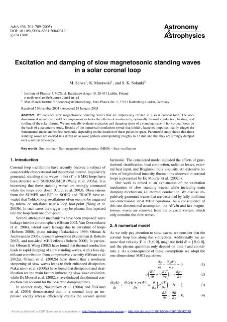
A&A 436, 701–709 (2005) 

DOI: 10.1051/0004-6361:20042319 

c○ ESO 2005 

Astronomy 

& 

Astrophysics 

Excitation and damping of slow magnetosonic standing waves 

in a solar coronal loop 

M. Selwa 1 ,K.Murawski 1 , and S. K. Solanki 2 

1 Institute of Physics, UMCS, ul. Radziszewskiego 10, 20-031 Lublin, Poland 

e-mail: mselwa@kft.umcs.lublin.pl 

2 Max-Planck-Institut für Sonnensystemforschung, Max-Planck-Str. 2, 37191 Katlenburg-Lindau, Germany 

Received 5 November 2004 / Accepted 24 January 2005 

Abstract. We consider slow magnetosonic standing waves that are impulsively excited in a solar coronal loop. The onedimensional 

numerical model we implement includes the effects of nonlinearity, optionally thermal conduction, heating, and 

cooling of the solar plasma. We numerically evaluate excitation and damping times of a standing wave in hot coronal loops on 

the basis of a parametric study. Results of the numerical simulations reveal that initially launched impulses mainly trigger the 

fundamental mode and its first harmonic, depending on the location of these pulses in space. Parametric study shows that these 

standing waves are excited in a dozen or so wave periods corresponding roughly to 13 min and that they are strongly damped 

over a similar time-scale. 

Key words. Sun: corona – Sun: magnetohydrodynamics (MHD) – Sun: oscillations 

1. Introduction 

Coronal loop oscillations have recently become a subject of 

considerable observational and theoretical interest. Impulsively 

generated, standing slow waves in hot (T > 6 MK) loops have 

been detected with SOHO/SUMER (Wang et al. 2003a). It is 

interesting that these standing waves are strongly attenuated 

while the loops cool down (Curdt et al. 2003). Observations 

from the SUMER and EIT on SOHO and TRACE have revealed 

that Yohkoh loop oscillations often seem to be triggered 

by micro- or sub-flares near a loop foot-point (Wang et al. 

2003b). In such cases the trigger may be plasma flow injected 

into the loop from one foot-point. 

Several attenuation mechanisms have been proposed: wave 

leakage into the chromosphere (Ofman 2002; Van Doorsselaere 

et al. 2004), lateral wave leakage due to curvature of loops 

(Roberts 2000), phase mixing (Nakariakov 1999; Ofman & 

Aschwanden 2002), resonant absorption (Ruderman & Roberts 

2002), and non-ideal MHD effects (Roberts 2000). In particular, 

Ofman & Wang (2002) have found that thermal conduction 

leads to rapid damping of slow standing waves, with a less significant 

contribution from compressive viscosity (Ofman et al. 

2002a). Ofman et al. (2002b) have shown that a nonlinear 

steepening of slow waves leads to their enhanced dissipation. 

Nakariakov et al. (2000a) have found that dissipation and stratification 

are the main factors influencing slow wave evolution, 

while De Moortel et al. (2002a) have deduced that thermal conduction 

can account for the observed damping times. 

In another study, Nakariakov et al. (2004) and Tsiklauri 

et al. (2004) demonstrated that in a coronal loop an impulsive 

energy release efficiently excites the second spatial 

harmonic. The considered model included the effects of gravitational 

stratification, heat conduction, radiative losses, external 

heat input, and Braginskii bulk viscosity. An extensive review 

of longitudinal intensity fluctuations observed in coronal 

loops is presented by De Moortel et al. (2002b). 

Our work is aimed at an explanation of the excitation 

mechanism of slow standing waves, while including main 

damping mechanism, i.e. thermal conduction. We discuss impulsively 

generated waves that are described by fully nonlinear 

one-dimensional ideal MHD equations. As a consequence of 

this one-dimensional assumption, the Alfvén and fast magnetosonic 

waves are removed from the physical system, which 

only contains the slow waves. 

2. A numerical model 

As we only pay attention to slow waves, we consider that the 

coronal loop lies along the x-direction. Additionally we assume 

that velocity V = [V, 0, 0], magnetic field B = [B, 0, 0], 

and the plasma quantities only depend on time t and coordinate 

x. As a consequence of these assumptions we adopt the 

one-dimensional MHD equations: 

∂ϱ 

∂(ϱE) 

∂t 

+ ∂[(ϱE + p T)V] 

∂x 

∂t + ∂(ϱV) = 0, (1) 

∂x 

∂t + V ∂V ) 

= − ∂p T 

∂x ∂x , (2) 

( ∂V 

ϱ 

= ∂ ∂x 

( 

σ ∂T 

∂x 

∂B 

∂t 

) 

+ H−L, (3) 

= ∂B 

∂x 

= 0. (4) 

Article published by EDP Sciences and available at http://www.edpsciences.org/aa or http://dx.doi.org/10.1051/0004-6361:20042319

702 M. Selwa et al.: Waves in coronal loops 

Here ϱ is the mass density, T – the temperature, and the symbol 

p T denotes a total pressure that represents the sum of the gas 

and magnetic pressures: 

) 

p T = 

(p + B2 

, (5) 

2µ 

where µ is the magnetic permeability. E is the plasma energy 

density: 

E = ϱV2 

2 + p T 

γ − 1 , (6) 

where γ is the adiabatic index. Coefficient σ corresponds to 

the thermal conductivity that follows from the formulation of 

Spitzer (1962) 

σ = κT 5/2 , (7) 

where κ = 9.2 × 10 −7 erg cm −1 s −1 K −7/2 is the plasma thermal 

conductivity. 

In Eq. (3) L represents a cooling term due to radiative 

losses from an optically thin plasma (Raymond 1978) and H 

is the heating term that is implemented phenomenologically as 

(Zingale et al. 2002) 

⎡ 

H = H 0 exp ⎢⎣− (x − x ⎤ 

0) 2 ( 

⎥⎦ exp − t ) 

· (8) 

2w 2 τ 

h 

We choose and fix the width of the heating source w h = 1.25 × 

10 8 cm, H 0 = 0.2ergcm −3 s −1 , the duration τ = 41 s, while the 

spatial position of heat deposition x 0 is left as a free parameter. 

These values correspond to parameters of a typical solar flare 

according to Nakariakov et al. (2004). 

2.1. The loop equilibrium 

We consider the equilibrium at which pressure p 0 = c 2 s ϱ 0 /γ = 

const. and plasma is at rest, V 0 = 0. We choose equilibrium 

density profile ϱ 0 , which varies with x such that ϱ 0 attains large 

values at loop foot-points settled at x = 0andx = L, where 

L = 50 × 10 8 cm is the loop length which corresponds to loop 

radius of 13−16 Mm. The loop is relatively short because short 

loops are easier to simulate. In Sect. 3.2 we also consider loops 

with other lengths. The mass density profile ϱ 0 (x) is similar to 

the profile implemented by Ofman (2002), i.e. 

{ } 

d 

ϱ 0 (x) = ϱ c 

2 [tanh (s (x − x tr) · (x − L + x tr )) + 1] + 1 · (9) 

Here d is the ratio of the photospheric mass density ϱ ph to 

coronal mass density ϱ c = 10 −15 gcm −3 . We allow this parameter 

to vary in the range 10 4 ≤ d ≤ 10 8 . The quantity 

s = 0.5×10 −17 cm −1 denotes the slope of ϱ 0 (x) at the loop footpoints, 

and x tr = 0.2842×10 8 cm corresponds to the position of 

the transition region. According to Eq. (9) ϱ 0 jumpsatthislocation. 

As T 0 (x) ∼ p 0 /ϱ 0 (x), the plasma temperature T 0 is higher 

at the solar corona than at the foot-points. We also choose the 

sound speed in the solar corona c s = √ γp 0 /ϱ 0 (x = L/2) = 

0.35 × 10 8 cm s −1 . 

2.2. Perturbations 

For the coronal loop that is described by Eqs. (1)–(3), perturbations 

can be excited in such a loop in numerous ways. Here we 

focus our attention on impulsively excited waves. We launch a 

hot pulse in the mass density, pressure, and velocity. This pulse 

has the following form: 

δϱ(x, t = 0) = A ϱ exp [ −(x − x 0 ) 2 /w 2] , (10) 

δp(x, t = 0) = A p exp [ −(x − x 0 ) 2 /w 2] , (11) 

δV(x, t = 0) = A V exp [ −(x − x 0 ) 2 /w 2] , (12) 

where A ϱ , A p ,andA V are initial amplitudes of the pulse, x 0 its 

initial position, and w its initial width. 

2.3. Analytical formulae for standing waves 

To derive analytical formulae for standing waves, we replace 

the profile of Eq. (9) by a uniform profile ϱ 0 = const., then 

neglect thermal conduction, heating, and cooling by setting 

σ = H = L = 0 in Eq. (3). Additionally we assume solidwall 

boundary conditions at x = 0andx = L by setting V = 0 

there. In this case initial perturbations after a sufficiently long 

time excite the standing wave oscillations given by the analytical 

formulae: 

V(x, t) = A v cos(ω n t)sin(k n x), (13) 

δϱ(x, t) = − ϱ 0A v 

c s 

sin(ω n t)cos(k n x), (14) 

δp(x, t) = −ϱ 0 A v c s sin(ω n t)cos(k n x), (15) 

where: 

k n = nπ L , ω n = c s k n . (16) 

Notice that perturbed mass density δϱ and velocity V display a 

phase shift of a quarter wave period. 

3. Numerical results 

In this part of the paper we present numerically obtained results 

for various run parameters. The plasma equations are solved 

numerically with the FLASH code (Fryxell et al. 2000). For 

most numerical runs 300 blocks are chosen. Each block contains 

8 grid cells. We performed grid convergence studies to 

verify that the numerical diffusion is negligibly small. Free 

boundary conditions are used at the boundaries of the simulation 

region, and all physical quantities are measured in cgs 

units. 

We discuss the fundamental mode and the first harmonic, 

which are both triggered by temperature perturbations and go 

on to pay particular attention to excitation and damping times 

of these modes. Our simulations show that these lowest modes 

are the dominantly excited ones for the pulse parameters employed. 

3.1. Excitation by temperature perturbation 

We now consider the case of ideal plasma for which there is 

no thermal conduction, cooling, and heating. This implies that 


M. Selwa et al.: Waves in coronal loops 703 

Fig. 2. Spatial profiles of velocity V(x, t = 18.842 T 1 )(left top panel), 

V(x, t = 19.274 T 1 )(left bottom panel), V(x, t = 37.841 T 2 )(right top 

panel), and V(x, t = 38.281 T 2 )(right bottom panel) for mass density 

contrast d = 10 8 , pulse width w = L/40, pulse position x 0 = L/4 (left 

panels), and x 0 = L/2 (right panels). Left (right) profiles correspond 

to the fundamental (first harmonic) mode. 

Fig. 1. Evolution of velocity V(x = L/4, t) (top panel) and mass density 

ϱ(x = L/4, t) (bottom panel) for mass density contrast d = 10 8 , 

pulse width w = L/40, and initial pulse position x 0 = L/4. 

the source terms on the right hand side of Eq. (3) are set to 

zero. So, we have σ = L = H = 0. Additionally we assume 

that there are no initial velocity perturbations. In this case slow 

waves are excited solely by temperature perturbations given by 

Eqs. (10)–(12) with A ϱ = 0.125 ϱ 0 (x 0 ), A p = 0.25 p 0 ,andA V = 

0. We launch the pulses of Eqs. (10)–(11) with a width of w = 

L/40, which is a typical value determined from observations 

(Nakariakov et al. 2004). We also carry out a parametric study 

in which parameters are allowed to vary around the adopted 

fiducial values. First we consider in some detail three cases that 

correspond to different positions of the initial pulses: (a) x 0 = 

L/4; (b) x 0 = L/2; (c) x 0 = 0. 

3.1.1. Time evolution of the pulses 

The basic time-signature of the excited mode is similar to 

a damped oscillation (see Fig. 1). However, the wave form 

evolves significantly with time. At the initial stages of evolution 

and in addition to the signal that is typical of standing mode, 

we observe some short-wave oscillations (Fig. 1), also seen in 

FFT spectra – not shown – and in wavelet spectra (Fig. 4). At 

later times the signal becomes almost sinusoidal. 

3.1.2. Pulses at a quarter of the loop length 

and at the apex of the loop 

If the initial pulse is launched at x 0 = L/4 (x 0 = L/2), the fundamental 

(first harmonic) mode is excited. Figure 2 displays 

spatial profiles of these waves at given moments in time. As the 

fundamental standing wave is twice longer than its harmonic 

(Fig. 2), the fundamental wave is less sensitive to the inhomogeneous 

medium, and essentially it occupies the cavity over 

all its length L. The harmonic wave is more sensitive to the 

Fig. 3. Time-signatures of perturbed mass density δϱ(x = L/4, t) (solid 

line) and velocity V(x = L/4, t) (dashed line) for d = 10 8 , w = L/40, 

x 0 = L/4(top panel), and x 0 = L/2(bottom panel). 

inhomogeneity than the fundamental wave, resulting in enhanced 

energy leakage into the photosphere. 

Time-signatures of perturbed mass density δϱ and velocity 

V, which are detected at spatial point x = L/4, are shown 

in Fig. 3 for a time after the initial high frequency power has 

died away. Oscillation amplitudes decrease with time as a consequence 

of wave damping due to energy leakage into the photosphere. 

In all considered cases the presence of the standing wave 

in the system is evaluated on the basis of normalized phase 

shift δφ, for the fundamental (n = 1) or harmonic (n = 2) 

standing waves. We establish an excitation criterion according 

to which a standing wave is present in the system if δφ departs 



T 

Wavelet Power Spectrum 

8 

16 

32 

64 

95% 

128 

95% 

256 

512 

95% 

0 5 10 15 20 

t/T 1 

T 


4 

8 

16 

32 

64 

128 

95% 

256 

512 

0 10 20 30 40 

t/T 2 

Fig. 4. Spectra of velocity V(x = L/4, t) from Fig. 3. The Fourier spectra 

are displayed in the top panels and the corresponding wavelet spectra 

in the bottom panels. Both the Fourier and wavelet analysis lead to 

wave periods T 1 ≈ 254 s, T 2 ≈ 125 s, where T n is the nth standing 

wave period. The hatched area in the lower frames indicate regions 

where the wavelet transform is less accurate. 

by 20% from 1/4, since the quarter period lag is a signature of 

the analytical solution of Sect. 2.3 , viz. 

1 

4 · 80% ≤ δφ ≤ 1 · 120%. (17) 

4 

This criterion is fulfilled for t > t min . As the standing wave excitation 

time we assume t min . According to this criterion the fundamental 

(harmonic) standing wave is excited at t ≈ 6 T 1 (t ≈ 

3.5T 2 ), where T 1 and T 2 are the analytically evaluated periods 

that are expressed by 

T n = 2L eff 

, (18) 

nc s 

where n denotes the standing wave number, c s – the sound 

speed, and L eff –theeffective loop length. From Fig. 2 we 

estimate that L eff ≈ 45 × 10 8 cm and then T 1 ≈ 257 s and 

T 2 ≈ 128 s. These values are close to the results of the fast 

Fourier transform (FFT) and wavelet analyses (Fig. 4). Small 

differences result from the fact that the effective length of the 

cavity is lower than L and differs for the case of n = 1and 

n = 2. Moreover, c s is an inhomogeneous function of x in our 

simulations, but is assumed to be x-independent when evaluating 

Eq. (18). 

We have restricted the Fourier analysis to t > 3 T 1 in order 

to remove the transient signal at the initial stage of temporal 

evolution. This signal is discernible in the wavelet power 

spectrum (Fig. 4) obtained using a Morlet mother function 

(Torrence & Compo 1998) 

ψ(η) = π −1/4 e imη e −η2 /2 

with m = 6. The wavelet transform was applied to the full time 

series. The solid contour represents 95% confidence, and the 

shaded area 90%. 

3.1.3. A pulse at a foot-point 

The initial pulse of Eqs. (10)–(11) is launched at the loop footpoint 

located at x = 0. Figure 5 displays the corresponding 

95% 

T 

32 

64 

128 


95% 

256 

95% 

512 

0 5 10 15 20 

t/T 1 

Fig. 5. A spatial velocity profile at t ≈ 20 T 1 (left top panel), timesignatures 

(right top panel) of the perturbed mass density δϱ(x = 

L/4, t) (solid line), and velocity V(x = L/4, t) (dotted line) for d = 10 8 , 

w = L/40, and x 0 = 0. The corresponding Fourier and wavelet power 

spectra are displayed in the bottom panels. 

results. As a result of a hot initial pulse, plasma is heated locally 

at the loop foot-point. Just warmed-up and dense photospheric 

plasma leaves the excitation region and fills up the 

coronal loop. As a consequence, δϱ grows in time (top right 

panels). The mean flow is directed to the loop center, and its 

efficiency declines both spatially in the region x > x 0 (left top 

panel) and with time (right top panel). Velocity power spectra 

(bottom panels) reveal the wave period of the fundamental 

standing wave T 1 . The background in the Fourier power spectrum 

is introduced by the velocity drift. The wave excitation 

time t ex ≈ 3 T 1 , and the damping time τ ≈ 5 T 1 . Qualitatively 

similar results have been obtained in the case of the initial 

pulse launched in the photosphere at x 0 = −L/50, i.e. outside 

the loop, corresponding to subsurface layers of the Sun (not 

shown). Recently Tsiklauri et al. (2004) discussed the case of 

heat deposition at a loop-foot point. 

3.1.4. Excitation of a packet of standing waves 

We excite different waves by setting the initial pulses in different 

parts of the loop. Fourier spectra show that an almost pure 

first harmonic standing wave is excited when the initial pulse 

is launched at the loop apex. In some cases we do not observe 

a single standing mode but instead a packet of modes in which 

the fundamental and harmonic standing modes make the largest 

contribution. Moving the excitation point from the loop apex 

to the foot-points results in an excitation of the fundamental 

mode. For the excitation points that are close to x 0 = L/2 we 

observe that the Fourier power in the first harmonic standing 

mode is much higher than in the fundamental standing mode, 

while for x 0 = 3L/8 the scenario changes and the fundamental 

mode dominates (Fig. 6). 

3.2. Parametric studies of wave excitation 

and damping times 

In this part of the paper we present results of parametric studies. 

We vary several parameters, such as pulse position x 0 ,density 

contrast d, pulse width w, temperature of initial pulses, and 

95% 



Fig. 6. Fourier spectra of the velocity V(x = L/4, t) ford = 10 8 , 

w = L/40, x 0 = 0.375L (top panel), and x 0 = 0.475L (bottom panel). 

Fundamental and the first harmonic standing modes are dominant in 

the top and bottom panels, respectively, but the first harmonic and fundamental 

modes are present there too. 

Fig. 7. Normalized standing wave excitation time t ex /T n (top panel) 

and normalized damping time τ/T n (bottom panel) vs. normalized 

pulse position x 0 /L for d = 10 8 and w = L/40. The squares (crosses) 

correspond to the fundamental (harmonic) standing waves. 

perturbations in velocity A V . We analyze how the standing 

wave excitation time t ex and damping time τ depend on these 

parameters. 

We first filter out non-oscillatory components from the 

time-signatures ϱ(x 0 = L/4, t) andV(x 0 = L/4, t) to remove 

trends, such as seen in the upper right panel of Fig. 5, and to get 

a pure signal that corresponds solely to oscillations. The filtering 

is done by the code originally developed by Ofman (2002). 

We estimate excitation time t ex with the criterion described by 

Eq. (17), while for damping time τ we fit an envelope of a 

velocity profile into the following formula 

( 

V(x = x d , t) = V 0 exp 

− t − t ex 

τ 

) 

, t ≥ t min , (19) 

where x d denotes the detection point, and V 0 is the amplitude 

of the velocity V at time t ex . 

We first consider the dependence of t ex and τ on the location 

x 0 of the initial pulse. Figure 7 shows that the fundamental 

(harmonic) standing wave excitation time t ex generally grows 

(declines) as the pulse position x 0 moves from the loop footpoint 

(x 0 = 0) to its apex (x 0 = L/2). In the case of the fundamental 

standing wave, the damping time depends weakly on 

x 0 with a slight tendency to decrease with x 0 (bottom panel of 

Fig. 7). The second standing wave damping time decreases as 

x 0 approaches L/2. 

These results support evidence that excitation and damping 

times are not constant but depend on the location of the initial 

pulse. Excitation time varies from its lowest value of 3 T 1 

for x 0 = 0 to its highest value of 16 T 1 for x 0 = 0.45 L for 

the fundamental standing wave (and from 3 T 2 for x 0 = L/2 

to 8 T 2 for x 0 = 0.45 L in the case of the second standing 

wave). The obtained values of damping time are in the 

range 4.7 T 1


Table 1. Excitation time t ex and damping time τ for two different 

widths of the pulse in the case of the second (n = 2) standing wave for 

d = 10 8 and x 0 = L/2. 

w/L t ex [s] τ [s] 

0.025 463 603 

0.6 1050 565 

Fig. 8. Normalized fundamental standing wave excitation time (top 

panel) and normalized damping time (bottom panel) vs.logd for w = 

L/40 and x 0 = L/4. 


panel) and damping factor (bottom panel) vs. normalized pulse temperature 

T r for d = 10 8 , w = L/40, and x 0 = L/4. 

Fig. 9. Normalized fundamental standing wave (n = 1) excitation time 

t ex /T n (top panel), and damping time τ/T n (bottom panel) vs. pulse 

width w for d = 10 8 and x 0 = L/4. 

function of x of the standing wave spatial profile of Eqs. (13)– 

(15); sufficiently wide pulses adjust faster to the standing 

waves. 

In the case of the second standing mode, its excitation and 

damping times vary with the pulse width (Table 1). For a very 

wide pulse the second standing wave is excited more slowely 

than by narrower pulses, but its damping time is slightly 

shorter. Note that, even for w = 3 × 10 9 cm, the initial pulse is 

close to the sine function of x and the second, not the fundamental, 

mode is excited for pulse position x 0 = L/2. 

So far, we have discussed the initial pulses of constant relative 

temperature T r = T p /T c = 1.1, where T p is the temperature 

of the initial pulse and T c is the temperature of the corona. This 

temperature is realized through the choice of pulse amplitudes 

A ϱ = 0.125ϱ 0 (x 0 )andA p = 0.25p 0 . It is worth quantifying 

an influence of T r on mode excitation time t ex and damping 

time τ. To do so, we consider three values of the temperature 

ratio: T r = 2(A ϱ = 0.125ϱ 0 (x 0 ), A p = 1.25p 0 ), T r = 4 

(A ϱ = 0.125ϱ 0 (x 0 ), A p = 3.5p 0 ), T r = 8(A ϱ = 0.125ϱ 0 (x 0 ), 

A p = 8.0p 0 ). Figure 10 summarizes results of the corresponding 

numerical experiments. According to our expectation a 

warmer pulse leads to more efficient standing wave excitation 

as the excitation time declines with T r ; a warmer pulse transfers 

itself in a shorter time to a sinusoidal standing wave profile. 

As a consequence of higher energy leakage, the standing wave 

is more rapidly damped for higher values of T r . Given that T r 

changes by a factor of 8, the induced changes in t ex and τ are 

relatively small (factor of 2). As warmer pulses correspond to 

higher amplitudes of the initial pulses we claim that nonlinearity 

does not play a vital role in affecting t ex and τ. 

We now compare four cases which correspond to the following 

loop lengths L 0 :(a)L 0 = L = 50 × 10 8 cm; (b) L 0 = 2L; 

(c) L 0 = 4L; and(d)L 0 = 6L. The pulse position was chosen 

as x 0 = L 0 /4. The normalized excitation time decreases with 

the loop length for narrow pulses (Fig. 11), and the damping 

time generally grows with loop length L 0 (right panel). Note 




panel) and damping time (bottom panel) vs. normalized loop length 

L 0 ,ford = 10 8 , x 0 = L 0 /4, and w = L/40. Note that T n now corresponds 

to the expected period for the appropriate loop length. 

Fig. 12. Normalized fundamental standing wave excitation time (left 

panel) and damping time (right panel) vs. the velocity amplitude of 

the initial pulse, A V ,ford = 10 8 , w = L/40, x 0 = L/4 (squares), and 

x 0 = L/2 (crosses). 

that since T n ∼ L 0 the results must be considered carefully, e.g. 

t ex actually grows with L 0 (in s). 

3.3. Velocity pulses 

In a similar case to the cases discussed above, the only difference 

is that to mass density and pressure perturbations we 

add a non-zero pulse in velocity. We choose and hold fixed 

A V = 0.125 c s (x 0 ). In the case of x 0 = L/4 the fundamental 

standing wave is generated at t ex ≈ 7 T 1 , which is a little larger 

than in the case of A V = 0 (Fig. 12). The damping time attains 

a value of τ ≈ 5.5 T 1 , which is 10% higher than without 

the velocity pulse. From this result we conclude that the fundamental 

mode is weakly damped while triggered by the velocity 

perturbations. 

In the case of both x 0 = L/2 and the harmonic standing 

wave (crosses) the excitation time is larger than in the case of 

A V = 0, while the damping time becomes a bit smaller than 

without the velocity pulse. The harmonic standing wave is excited 

in a longer lapse of time and is stronger damped while 

being excited by a velocity pulse. 

3.4. Perturbations of non-ideal plasma 

Next we consider several cases of non-ideal plasma with different 

effects switched on. In our approach we neglect background 

heating, which has been used by Nakariakov et al. (2004) to 

keep background temperature at the coronal value of ∼1 MK. 

Instead, we direct most of our attention to the effect of nonideal 

plasma on wave propagation. Table 2 summarizes all the 

results that are obtained for the width of the pulse W = L/40 

and its initial position x 0 = L/4. 

We discuss in some detail the case of thermal conduction, 

heating, and cooling acting simultaneously. In this case we do 

not observe a pure standing wave but instead a packet of waves 

with largest contribution from the fundamental standing wave 

(left bottom panel of Fig. 13). Mass density collected at x d = 

L/4 exhibits oscillations that decay in time. The mean value of 

the mass density grows in time as a result of thermal conduction 

(right top panel of Fig. 13). Velocity spectra reveal the mean 

period of T 1 = 410 s (bottom panels of Fig. 13). Note that this 

value is higher than in the case of the ideal plasma due to a 

= √ γp/ϱ that 

results from the cooling and thermal conduction (Fig. 14). 

It is noteworthy that thermal conduction acting alone excites 

a bunch of waves at the loop foot-points where the thermal 

conduction is mostly effective (not shown). The most significant 

value of standing wave period is similar to the case 

without conductivity. Taking both thermal conduction and heating 

into account leads to a significant increase in the period of 

the observed standing wave. In the case of thermal conduction 

switched on, evaporation of a photospheric plasma takes place. 

It is interesting, however, that it is not continuous but occurs in 

the form of parcels which propagate out of the photosphere in 

certain lapses of time with each separate from the other. 

This scenario can be explained as follows. Photospheric 

plasma gets heated due to thermal conduction. As this heated 

material is denser than a coronal plasma, a sufficient amount of 

heating is needed for a parcel of the photospheric gas to attain 

enough pressure to leave the photosphere. 

different value of the effective sound speed c eff 

s 

4. Summary 

In this paper we have considered the excitation and damping 

of slow standing waves in a solar coronal loop that is 



Table 2. Standing wave period T , excitation time t ex , and damping time τ for various run parameters in cgs units. The sign − means that a value 

could not be evaluated. 

A ϱ A p A V d c s [cm s −1 ] H L σ T [s] t ex [s] τ[s] 

0 0 =0 10 8 0.35 × 10 8 =0 =0 =0 254 1578 1250 

0 0 =0 10 8 0.35 × 10 8 0 =0 =0 208 915 986 

0 0 =0 10 8 0.35 × 10 8 0 0 =0 208 916 998 

=0 =0 =0 10 8 0.35 × 10 8 0 0 =0 208 919 1009 

=0 =0 =0 10 8 0.35 × 10 8 =0 =0 0 − − − 

0 0 =0 10 8 0.35 × 10 8 =0 =0 0 500 1291 2289 

0 0 =0 10 8 0.35 × 10 8 0 =0 0 556 1133 1178 

=0 =0 =0 10 4 0.35 × 10 8 =0 =0 0 278 − − 

0 0 =0 10 4 0.35 × 10 8 =0 =0 0 455 − − 

0 0 =0 10 8 0.1 × 10 8 =0 =0 =0 882 4627 3826 

0 0 =0 10 8 0.1 × 10 8 =0 =0 0 909 1113 3930 

0 0 =0 10 8 0.35 × 10 8 0 0 0 400 827 2170 

T 


4 

8 

16 

32 

64 

128 

256 

512 95% 

1024 

0 5 10 15 20 

t/T 1 

Fig. 13. A spatial velocity profile at t ≈ 12 T 1 (left top panel), the 

corresponding time-characteristics of mass density signal (right top 

panel), the Fourier spectrum (left bottom panel), and the wavelet spectrum 

(right bottom panel) ford = 10 8 , w = L/40, x 0 = L/4, σ 0, 

H 0, L 0, A ϱ 0, A p 0, and A V = 0. 

95% 

95% 

95% 

approximated by a one-dimensional plasma. Our model 

implements optionally thermal conduction, heating, cooling, 

and impulses in plasma quantities. The thermal conductivity 

follows the formulation of Spitzer (1962). The phenomenological 

heating source term is localized in space and time. Cooling 

is due to radiative losses from an optically thin plasma. A Fast 

Fourier transform and wavelet analysis of temporal wave profiles 

have shown that in a loop the fundamental or harmonic 

standing slow waves are excited depending on the location of 

the trigger. We worked out a simple criterion for the presence of 

a standing wave based on a phase shift between perturbed mass 

density δϱ and velocity V. The time required for a standing 

wave to settle in a loop from a hot initial pulse is of the order 

of a dozen or so wave periods and varies, depending on such 

parameters of the plasma as the initial location of the pulse, 

the density contrast, or the pulse width. In the case of a wide 

and strong pulse, as well as of heated plasma, this time-scale is 

shorter. 

The one-dimensional model we have developed obviously 

suffers from several drawbacks. Its main shortcoming is that 

Fig. 14. Effective sound speed at t = 0(top panel) andt = 5000 s 

(bottom panel) in the case of Fig. 13. 

it only takes slow magnetosonic waves into account and neglects 

the presence of fast and Alfvén waves in the system. 

As a consequence, this model excludes several likely damping 

mechanisms that were already suggested in the literature. 

However, these neglected effects are believed to be unimportant 

as far as the scenario of slow wave excitation and damping 

are concerned. More realistic models of slow wave development 

are currently under development and the results will be 

reported elsewhere. 

Acknowledgements. The authors express their thanks to the anonymous 

referee and to Dr. Luigi Nocera for their constructive comments 

on an earlier draft of this paper. The FLASH code is provided 

by ASCI (Alliances Center for Astrophysical Thermonuclear 

Flashes) at the University of Chicago. Wavelet software is disseminated 

by C. Torrence and G. Compo, and is available at 



URL http://paos.colorado.edu/research/wavelets. M.S.’s 

and K.M.’s work was financially supported by a grant from the State 

Committee for Scientific Research Republic of Poland, with KBN 

grant No. 2 PO3D 016 25. 

References 

Aschwanden, M., Fletcher, L., Schrijver, C., & Alexander, D. 1999, 

ApJ, 520, 880 

Curdt, W., Wang, T. J., Dammasch, T. E., & Solanki, S. K. 2003, Hvar 

Obs. Bull., 27, 83 

De Moortel, I., & Hood, A. W. 2003, A&A, 408, 755 

De Moortel, I., Hood, A. W., & Ireland, J. 2002a, A&A, 381, 311 

De Moortel, T., Hood, A. W., Ireland, J., & Walsh, R. W. 2002b, Sol. 

Phys., 209, 89 

Fryxell, B., Olson, K., Ricker, P., et al. 2000, ApJS, 131, 273 

Nakariakov, V. M., Ofman, L., DeLuca, E. E., Roberts, B., & Davila, 

J. M. 1999, Science, 285, 862 

Nakariakov, V. M., Verwichte, E., Berghmans, D., & Robbrecht, E. 

2000, A&A, 362, 1151 

Nakariakov, V. M., Tsiklauri, D., Kelly, A., Arber, T. D., & 

Aschwanden, M. J. 2004, A&A, 414, L25 

Ofman, L. 2002, ApJ, 568, L135 

Ofman, L., & Wang, T. J. 2002, ApJ, 580, L85 

Ofman, L., & Aschwanden, M. 2002, ApJ, 576, L153 

Ofman, L., Nakariakov, V. M., & Sehgal, N. 2000, ApJ, 533, 1071 

Roberts, B. 2000, Sol. Phys., 193, 139 

Ruderman, M. S., & Roberts, B. 2002, ApJ, 577, 475 

Spitzer, L. 1962, Physics of fully ionized gases (New York: Wiley) 

Torrence, C., & Compo, G. P. 1998, Bull. Amer. Meteor. Soc., 79, 61 

Tsiklauri, D., Nakariakov, V. M., Arber, T. D., & Aschwanden, M. J. 

2004, A&A, 422, 351 

Van Doorsselaere, T., Debosscher, A., Andries, J., & Poedts, S. 2004, 

A&A, 424, 1065 

Wang, T. J., Solanki, S. K., Curdt, W., Innes, D. E., & Dammasch, I. E. 

2002, ApJ, 574, L101 

Wang, T. J., Solanki, S. K., Innes, D. E., Curdt, W., & Marsch, E. 

2003a, A&A, 402, L17 

Wang, T. J., Solanki, S. K., Curdt, W., et al. 2003b, A&A, 406, 1105 

Zingale, M., Dursi, L. J., ZuHone, J., et al. 2002, ApJS, 143, 539

Excitation and damping of slow magnetosonic standing waves in a ...

You also want an ePaper? Increase the reach of your titles

Delete template?

Save as template?