A complete gradient clustering algorithm formed with kernel estimators

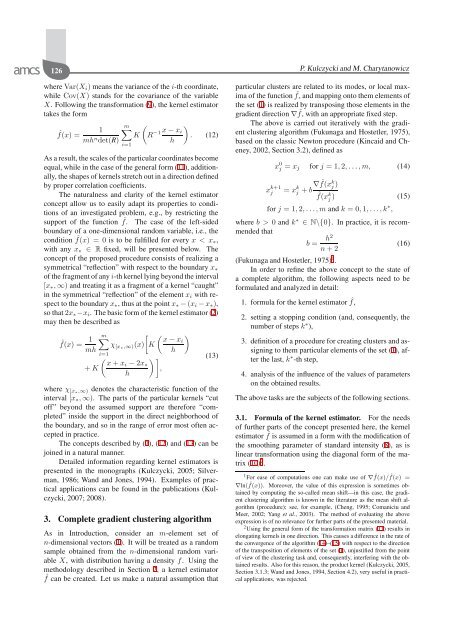
126 P. Kulczycki and M. Charytanowicz
where Var(X i ) means the variance of the i-th coordinate,
while Cov(X) stands for the covariance of the variable
X. Following the transformation (9), the kernel estimator
takes the form
ˆf(x) =
1
mh n det(R)
m∑
i=1
(
K R −1 x − x )
i
. (12)
h
As a result, the scales of the particular coordinates become
equal, while in the case of the general form (11), additionally,
the shapes of kernels stretch out in a direction defined
by proper correlation coefficients.
The naturalness and clarity of the kernel estimator
concept allow us to easily adapt its properties to conditions
of an investigated problem, e.g., by restricting the
support of the function ˆf. The case of the left-sided
boundary of a one-dimensional random variable, i.e., the
condition ˆf(x) =0is to be fulfilled for every x0 and k ∗ ∈ N\{0}. In practice, it is recommended
that
b =
h2
(16)
n +2
(Fukunaga and Hostetler, 1975) 1 .
In order to refine the above concept to the state of
a complete algorithm, the following aspects need to be
formulated and analyzed in detail:
1. formula for the kernel estimator ˆf,
2. setting a stopping condition (and, consequently, the
number of steps k ∗ ),
3. definition of a procedure for creating clusters and assigning
to them particular elements of the set (1), after
the last, k ∗ -th step,
4. analysis of the influence of the values of parameters
on the obtained results.
The above tasks are the subjects of the following sections.
3.1. Formula of the kernel estimator. For the needs
of further parts of the concept presented here, the kernel
estimator ˆf is assumed in a form with the modification of
the smoothing parameter of standard intensity (8), as is
linear transformation using the diagonal form of the matrix
(10) 2 .
1 For ease of computations one can make use of ∇ ˆf(x)/ ˆf(x) =
∇ln( ˆf(x)). Moreover, the value of this expression is sometimes obtained
by computing the so-called mean shift—in this case, the gradient
clustering algorithm is known in the literature as the mean shift algorithm
(procedure); see, for example, (Cheng, 1995; Comaniciu and
Meer, 2002; Yang et al., 2003). The method of evaluating the above
expression is of no relevance for further parts of the presented material.
2 Using the general form of the transformation matrix (11) results in
elongating kernels in one direction. This causes a difference in the rate of
the convergence of the algorithm (14)–(15) with respect to the direction
of the transposition of elements of the set (1), unjustified from the point
of view of the clustering task and, consequently, interfering with the obtained
results. Also for this reason, the product kernel (Kulczycki, 2005,
Section 3.1.3; Wand and Jones, 1994, Section 4.2), very useful in practical
applications, was rejected.