A complete gradient clustering algorithm formed with kernel estimators

130 P. Kulczycki and M. Charytanowicz
(a)
(b)
(c)
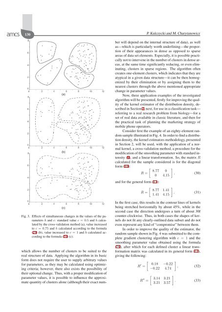
Fig. 3. Effects of simultaneous changes in the values of the parameters
h and c: standard value c =0.5 and h calculated
by the cross-validation method (a), value increased
to c =0.75 and h calculated according to the formula
(29) (b), value increased to c =1and h calculated according
to the formula (29) (c).
which allows the number of clusters to be suited to the
real structure of data. Applying the algorithm in its basic
form does not require the user to supply arbitrary values
for parameters, as they may be calculated using optimizing
criteria; however, there also exists the possibility of
their optional change. Thus, with a proper modification of
parameter values, it is possible to influence the approximate
quantity of clusters alone (although their exact number
will depend on the internal structure of data), as well
as—which is particularly worth underlining—the proportion
of their appearances in dense as opposed to sparse
areas of data set elements. Especially, it is possible practically
not to intervene in the number of clusters in dense areas,
at the same time significantly reducing, or even eliminating,
clusters in sparse regions. The algorithm often
creates one-element clusters, which indicates that they are
atypical in a given data structure—it can be then homogenized
by their elimination or by assigning them to the
nearest clusters through the above mentioned appropriate
change in parameter values.
Now, three application examples of the investigated
algorithm will be presented, firstly for improving the quality
of the kernel estimator of the distribution density, described
in Section 2, next, for use in a classification task—
referring to a real research problem from biology—for a
set of real data available in classic literature, and then for
the practical task of planning the marketing strategy of
mobile phone operators.
Consider first the example of an eighty-element random
sample illustrated in Fig. 4. In order to find a distribution
density, the kernel estimators methodology, presented
in Section 2, will be used, with the application of a normal
kernel, a cross-validation method, a procedure for the
modification of the smoothing parameter with standard intensity
(8), and a linear transformation. So, the matrix R
calculated for the sample considered is for the diagonal
form (10):
R =
[ 8.77 0
0 4.15
and for the general form (11):
[
8.77 1.41
R =
1.41 4.15
]
, (30)
]
. (31)
In the first case, this results in the contour lines of kernels
being stretched horizontally by about 45%, while in the
second case the direction undergoes a turn of about 30ř
counter-clockwise. Thus, in both cases the shapes of kernels
do not fit any clearly-outlined data subset and do not
even represent any kind of “compromise” between them.
In order to improve the quality of the estimator, the
random sample shown in Fig. 4 was submitted to the complete
gradient clustering algorithm with c = 1 and the
smoothing parameter value obtained using the formula
(29), after which for each defined cluster a linear transformation
matrix was calculated in its general form (11),
giving the following:
R ′ =
R ′′ =
[ 0.18 −0.22
−0.22 4.74
[ 3.14 3.21
3.21 3.57
]
, (32)
]
. (33)