A multi-factor model for the valuation and risk management of ...

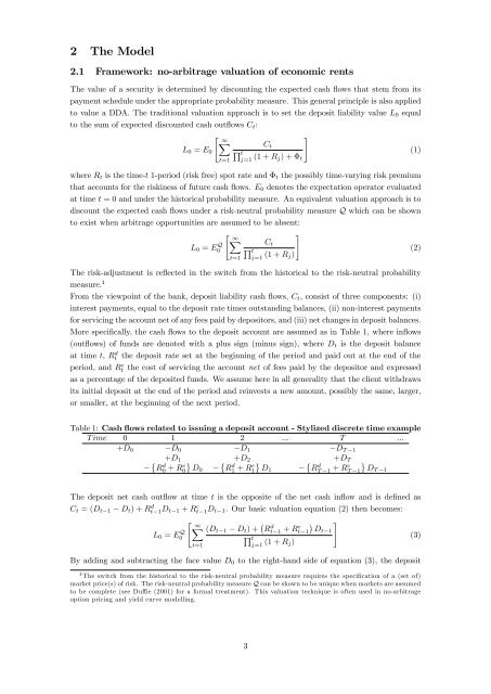
2 The Model
2.1 Framework: no-arbitrage valuation of economic rents
The value of a security is determined by discounting the expected cash ‡ows that stem from its
payment schedule under the appropriate probability measure. This general principle is also applied
to value a DDA. The traditional valuation approach is to set the deposit liability value L 0 equal
to the sum of expected discounted cash out‡ows C t :
" 1
#
X C t
L 0 = E 0 Q t
j=1 (1 + R (1)
j) + t
t=1
where R t is the time-t 1-period (risk free) spot rate and t the possibly time-varying risk premium
that accounts for the riskiness of future cash ‡ows. E 0 denotes the expectation operator evaluated
at time t = 0 and under the historical probability measure. An equivalent valuation approach is to
discount the expected cash ‡ows under a risk-neutral probability measure Q which can be shown
to exist when arbitrage opportunities are assumed to be absent:
L 0 = E Q 0
" 1
X
t=1
C t
Q t
j=1 (1 + R j)
The risk-adjustment is re‡ected in the switch from the historical to the risk-neutral probability
measure. 4
From the viewpoint of the bank, deposit liability cash ‡ows, C t , consist of three components: (i)
interest payments, equal to the deposit rate times outstanding balances, (ii) non-interest payments
for servicing the account net of any fees paid by depositors, and (iii) net changes in deposit balances.
More speci…cally, the cash ‡ows to the deposit account are assumed as in Table 1, where in‡ows
(out‡ows) of funds are denoted with a plus sign (minus sign), where D t is the deposit balance
at time t, Rt
d the deposit rate set at the beginning of the period and paid out at the end of the
period, and Rt c the cost of servicing the account net of fees paid by the depositor and expressed
as a percentage of the deposited funds. We assume here in all generality that the client withdraws
its initial deposit at the end of the period and reinvests a new amount, possibly the same, larger,
or smaller, at the beginning of the next period.
#
(2)
Table 1: Cash ‡ows related to issuing a deposit account - Stylized discrete time example
T ime 0 1 2 ... T ...
+D 0 D 0 D 1 D T 1
+D 1 +D 2 +D T
R
d
0 + R c 0 D 0
R
d
1 + R c 1 D 1
R
d
T 1 + R c T 1 D T 1
The deposit net cash out‡ow at time t is the opposite of the net cash in‡ow and is de…ned as
C t = (D t 1 D t ) + R d t 1D t 1 + R c t 1D t 1 . Our basic valuation equation (2) then becomes:
L 0 = E Q 0
" 1
X
t=1
(D t 1 D t ) + R d t 1 + R c t 1
Dt 1
Q t
j=1 (1 + R j)
By adding and subtracting the face value D 0 to the right-hand side of equation (3), the deposit
4 The switch from the historical to the risk-neutral probability measure requires the speci…cation of a (set of)
market price(s) of risk. The risk-neutral probability measure Q can be shown to be unique when markets are assumed
to be complete (see Du¢ e (2001) for a formal treatment). This valuation technique is often used in no-arbitrage
option pricing and yield curve modelling.
#
(3)
3