The Euclid Abstract Machine: - Centro de Matemática e Aplicações ...

The Euclid Abstract Machine:
Trisection of the Angle and the Halting Problem
Jerzy Mycka 1⋆ , Francisco Coelho 2 , and José Félix Costa 3
1 Institute of Mathematics,
University of Maria Curie-Sklodowska
Lublin, Poland
Jerzy.Mycka@umcs.lublin.pl
2 Department of Mathematics,
Universidade de Évora, Portugal
fcoelho@uevora.pt
3 Department of Mathematics,
I.S.T., Universidade Técnica de Lisboa
and CMAF – Centro de Matemática e Aplicações Fundamentais,
Lisboa, Portugal
fgc@math.ist.utl.pt
He took the golden Compasses, prepar’d
In Gods Eternal store, to circumscribe
This Universe, and all created things:
One foot he center’d, and the other turn’d
Round through the vast profunditie obscure,
And said, thus farr extend, thus farr thy bounds,
This be thy just Circumference, O World.
Milton, Paradise Lost
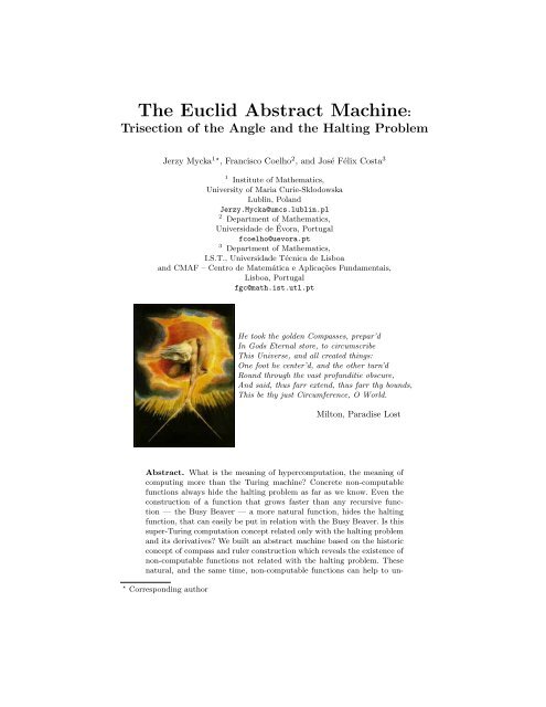
Abstract. What is the meaning of hypercomputation, the meaning of
computing more than the Turing machine? Concrete non-computable
functions always hide the halting problem as far as we know. Even the
construction of a function that grows faster than any recursive function
— the Busy Beaver — a more natural function, hides the halting
function, that can easily be put in relation with the Busy Beaver. Is this
super-Turing computation concept related only with the halting problem
and its derivatives? We built an abstract machine based on the historic
concept of compass and ruler construction which reveals the existence of
non-computable functions not related with the halting problem. These
natural, and the same time, non-computable functions can help to un-
⋆ Corresponding author

derstand the nature of the uncomputable and the purpose, the goal, and
the meaning of computing beyond Turing.
1 Operations
Let us imagine a construction of algorithms acting in the framework of Euclid’s
geometry. We can use an infinite (in reality sufficiently large) sheet of paper,
an unmarked ruler and a compass. Now we need to specify the list of possible
operations.
– P (P 1 , . . . , P n ) — Draw a finite number of distinct points P 1 , . . . , P n . 4
– C(P, Q) — Draw the circle with the center P and going through the point
Q.
– LC(P, Q; A) — Give the label A to the circle with the center P and going
through the point Q.
– L(P, Q) — Draw the line passing through P and Q.
– LL(P, Q; A) — Give the label A to the line passing through P and Q.
– LP (O 1 , O 2 ; A, B) — Give the label A to the point of the intersection of the
objects (lines or circles) O 1 and O 2 , in the case of two intersections choose
freely the order of labeling by A and B.
– D(A) — Delete the label A.
– X ∈ C : n — If the point X is in the circle C, then execute the n-th
instruction; otherwise go to the next instruction.
Of course, from the first operation we see that points are always labeled,
unless labels are ultimately removed through a D instruction. Let us add that
each label can be used only in the unique way, i.e., one label can identify exactly
one object. This does not mean that some objects cannot have two or more
labels.
A program is a numbered list of operations of the above types. After the n-th
operation the next one (with the number n + 1) is executed, unless it is the last
operation or it is the test operation X ∈ C : n.
Example 1.1. Let us consider the construction of two perpendicular lines. We
need to start with two points P, Q, then draw the line through these points.
Next we need two circles to construct a perpendicular line. Here is the code.
01 :: P (P, Q)
02 :: L(P, Q)
03 :: LL(P, Q; A)
04 :: C(P, Q)
05 :: LC(P, Q; C)
06 :: D(Q)
4 We can think about this operation as a weak version of the choice axiom – we can
always choose finite set of different points from Euclidean plane.

07 :: LP (A, C; Q 1 , Q 2 )
08 :: C(Q 1 , Q 2 )
09 :: LC(Q 1 , Q 2 , C 1 )
10 :: C(Q 2 , Q 1 )
11 :: LC(Q 2 , Q 1 , C 2 )
12 :: LP (C 1 , C 2 ; S 1 , S 2 )
13 :: L(S 1 , S 2 )
By the similarly constructed programs we can give Euclid machines, which
draw equilateral triangles or a bisector of some angle.
Let us consider an analogy which exists between programs of Euclid machines
and theorems of Euclidean geometry.
Example 1.2. We can start by recalling Thales’ Theorem: An inscribed angle in
a semicircle is a right angle. How can this fact be checked by means of Euclid
machines. Let us imagine the following construction.
– Draw three different, non-colinear points O, A, X.
– Draw the circle C with the center O and going through A; draw the line L
through O and A, label the point of intersection of L and C by B.
– Draw the line through O and X, label the other point of the intersection of
this line and C as P .
– Draw two lines: the first one going through A and P ; the second one going
through B and P .
– Draw the perpendicular L ′ for the line BP going by P .
– Label the intersection of L ′ and L as A ′ .
Now let us analyze the above part of the program (which can be translated
into instructions of the Euclid machine in the obvious manner). We have constructed
the angle ∠AP B and, after that, we have added the perpendicular L ′
to P B in the point P . Thus the fact that ∠AP B is a right angle is equivalent to
the fact that the points A (the intersection of AP with L) and A ′ (the intersection
of L ′ and L are identical. We can use the test operation to check the last
statement, let us assume that every point is a circle with a radius of the length
0.
– A ′ ∈ A : n
We can use this situation to build some kind of output. For example, the
program would end its activity if this condition is true; otherwise it would go
into infinite loop. Or we can draw some previously chosen labels for some point
(e.g. O): + for the positive test; − for the negative one.
In the light of the above example we can translate proposed proofs of Euclidean
geometry in equivalent programs; the proof is correct if for all initial
configurations we obtain the previously chosen special sign (e.g., +) of an acceptance.

2 URM machines
In this section we present the Turing completeness of the above described geometrical
machine. We use for this purpose the unlimited register machine [3]
(URM). Every unlimited register machine program is a finite sequence of instructions
acting on (potentially) infinite number of registers containing natural
numbers. The instructions of URM machines programs can be chosen in the
following way.
– Z(n) — Put 0 into the n-th register.
– S(n) — Increment the current value of the n-th register.
– J(n, m, k) — If the values in the n-th and m-th registers are equal, jump to
the k-th instruction.
2.1 The emulation of registers
Let us consider a program P of some URM machine, and let r be a number of
registers used in this program. Then we will use a pencil of r lines to emulate
these registers. The construction will be done in the following way.
– Draw two distinct points P, Q.
– Draw the line through P and Q.
– Label this line as R 1 .
– Draw the perpendicular to R 1 in P .
– Label this perpendicular as R n .
– Construct the bisector of R 1 and R n .
– Label it as R n−1 .
– Construct the consecutive bisectors of R 1 and R n−1 , R n−2 , . . . , R 2 and label
them as R n−2 , . . . , R 1 .
– Draw the circle with the center P and going through the point Q.
– Label this circle as C.
– Label the intersections of C and R 1 , . . . , R n as X 1 , Y 1 , . . . , X n , Y n .
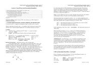
The line R i is used to remember values of the i-th register. The distance of
point X i to P , where X i , lying in the circle, informs us about the current value
|P Q|
which is equal to log 2 |P X i|
. In the case we need to put zero into some register
we should move the point X i to the intersection of R i and C again.
Let us add an important remark. During the whole computation (or rather
drawing) the labels of the main elements of our system, i.e., the starting points
P , Q, register lines R 1 , ..., R n , and the circle C will be not removed or changed.

R4
R3
R2
C
✏
X4
✬✩ X3 X2
P X1=Q
R1
✫✪
✏ ✏✏✏✏✏✏✏✏✏✏✏✏✏✏✏✏✏✏✏✏✏✏✏ ✱ ✱✱✱✱✱✱✱✱✱✱✱✱✱✱✱✱✱✱
Fig. 1. Simulation of 4 registers
P
X1”(=2) X1’(=1)
Q=X1(=0)
Fig. 2. Values in one register
2.2 The translation of URM instructions
Let us describe the translation of URM instructions into operations of Euclid
machines
Z(n): move the point X n to the intersection of R n and C
k :: D(X n )
k + 1 :: LP (R n , C; X n )
S(n): divide the segment P X n into two subsegments with the same length and
label the center point as X n
k :: C(P, X n )
k + 1 :: LC(P, X n ; C 1 )
k + 2 :: C(X n , P )
k + 3 :: LC(X n , P ; C 2 )
k + 4 :: LP (C 1 , C 2 ; P 1 , P 2 )
k + 5 :: L(P 1 , P 2 )

k + 6 :: LL(P 1 , P 2 ; L)
k + 7 :: D(X n )
k + 8 :: LP (L, R n ; X n )
k + 9 :: D(C 1 )
k + 10 :: D(C 2 )
k + 11 :: D(P 1 )
k + 12 :: D(P 2 )
k + 13 :: D(L)
J(n, m, s): test whether the point X n is in the circle with the center P and the radius
P X m and whether the point X m is in the circle with the center P and the
radius P X n
k :: C(P, X n )
k + 1 :: LC(P, X n ; C n )
k + 2 :: C(P, X m )
k + 3 :: LC(P, X m ; C m )
k + 4 :: X n ∈ C m : k + 6
k + 5 :: P ∈ C : k + 7
k + 6 :: X m ∈ C n : k + 10
k + 7 :: D(C n )
k + 8 :: D(C m )
k + 9 :: P ∈ C : k + 13
k + 10 :: D(C n )
k + 11 :: D(C m )
k + 12 :: P ∈ C : s ′
where s ′ is the starting number of the Euclid corresponding instruction,
equivalent to the s-th instruction of the URM machine.
Note that, in the machine above, we used the unconditional jumping instruction
P ∈ C. This unconditional jumping could have been translated directly
from the URM language into an appropriate geometrical instruction.
2.3 Euclid machines are Turing complete
Let us add the we have to proceed with the re-enumeration of the instructions
due to the fact that every Z instruction needs 2 operations, every S instruction
needs 14 operations and J needs 13 operations. With this re-enumeration we
have a complete description how to translate any URM machine into some
Euclid machine. So, we obtain the following proposition.
Proposition 2.1. Every URM machine can be simulated by some Euclid machine.
Example 2.1. Let us start with the simple example of the sum of two natural
numbers. We start with a preparation of 3 lines R 1 , R 2 , R 3 of the same pencil
with the center P , and the circle C going through these lines with the points of
intersections called X 1 , X 2 , X 3 .

\\ draw the line R 1
01 :: P (P, Q)
02 :: L(P, Q)
03 :: LL(P, Q; R 1 )
04 :: C(P, Q)
05 :: LC(P, Q; C)
06 :: D(Q)
07 :: LP (R 1 , C; X 1 , Y 1 )
\\ draw the perpendicular
line R 3
08 :: C(X 1 , Y 1 )
09 :: LC(X 1 , Y 1 , C 1 )
10 :: C(Y 1 , X 1 )
11 :: LC(Y 1 , X 1 , C 2 )
12 :: LP (C 1 , C 2 ; S 1 , S 2 )
13 :: L(S 1 , S 2 )
14 :: LL(S 1 , S 2 , R 3 )
15 :: D(C 1 )
16 :: D(C 2 )
17 :: D(S 1 )
18 :: D(S 2 )
19 :: D(Y 1 )
20 :: LP (R 3 , C; X 3 , Y 3 )
21 :: D(Y 3 ),
\\ draw the bisector of
the angle R 3 , P, R 1 and
call it R 2
22 :: C(X 1 , P )
23 :: LC(X 1 , P ; C 1 )
24 :: C(X 3 , P )
25 :: LC(X 3 , P ; C 3 )
26 :: LP (C 1 , C 3 ; S 1 , S 2 )
27 :: L(S 1 , S 2 )
28 :: LL(S 1 , S 2 , R 2 )
29 :: D(S 1 )
30 :: D(S 2 )
31 :: D(C 1 )
32 :: D(C 3 )
33 :: LP (R 2 , C; X 2 , Y 2 )
34 :: D(Y 2 )
To start a computation for some n, m ∈ N we need to place the points
X 1 , X 2 on the lines R 1 , R 2 in such a way that the following conditions hold:
|P X 1 | = |P X′ 1 |
2
, |P X n 2 | = |P X′ 2 |
2
, where X 0, ′ X ′ m 1 represent the initial position of
X 1 , X 2 . For this purpose we need to use n times the operation S(1) and m times
the operation S(2).
We can use the following URM machine program to implement the problem
of an addition. We assume the arguments are in the registers 1 and 2; the rest
of registers is initially equal to zero.
1 : J(2, 3, 6)
2 : S(1)
3 : S(3)
4 : J(2, 3, 6)
5 : J(1, 1, 2)
Now this sequence of the URM instructions can be translated into operations
of the Euclid machine in the following manner.
\\J(2, 3, 6)
01 :: C(P, X 2 )
02 :: LC(P, X 2 ; C 2 )
03 :: C(P, X 3 )
04 :: LC(P, X 3 ; C 3 )
05 :: X 2 ∈ C 3 : 7
06 :: P ∈ C : 8
07 :: X 3 ∈ C 2 : 11
08 :: D(C 2 )
09 :: D(C 3 )
10 :: P ∈ C : 14
11 :: D(C 2 )
12 :: D(C 3 )
13 :: P ∈ C : 68
\\S(1)
14 :: C(P, X 1 )
15 :: LC(P, X 1 ; C 1 )
16 :: C(X 1 , P )
17 :: LC(X 1 , P ; C 2 )
18 :: LP (C 1 , C 2 ; P 1 , P 2 )
19 :: L(P 1 , P 2 )
20 :: LL(P 1 , P 2 ; L)
21 :: D(X 1 )
22 :: LP (L, R 1 ; X 1 )
23 :: D(C 1 )
24 :: D(C 2 )
25 :: D(P 1 )
26 :: D(P 2 )
27 :: D(L)
\\S(3)
28 :: C(P, X 3 )
29 :: LC(P, X 3 ; C 1 )
30 :: C(X 3 , P )
31 :: LC(X 3 , P ; C 2 )
32 :: LP (C 1 , C 2 ; P 1 , P 2 )
33 :: L(P 1 , P 2 )
34 :: LL(P 1 , P 2 ; L)
35 :: D(X 3 )
36 :: LP (L, R 3 ; X 3
37 :: D(C 1 )
38 :: D(C 2 )
39 :: D(P 1 )

40 :: D(P 2 )
41 :: D(L)
\\J(2, 3, 6)
42 :: C(P, X 2 )
43 :: LC(P, X 2 ; C 2 )
44 :: C(P, X 3 )
45 :: LC(P, X 3 ; C 3 )
46 :: X 2 ∈ C 3 : 48
47 :: P ∈ C : 49
48 :: X 3 ∈ C 2 : 52
49 :: D(C 2 )
50 :: D(C 3 )
51 :: P ∈ C : 55
52 :: D(C 2 )
53 :: D(C 3 )
54 :: P ∈ C : 68
\\J(1, 1, 2)
55 :: C(P, X 1 )
56 :: LC(P, X 1 ; C 1 )
57 :: C(P, X 1 )
58 :: LC(P, X 1 ; C 1 )
59 :: X 1 ∈ C 1 : 61
60 :: P ∈ C : 62
61 :: X 1 ∈ C 1 : 65
62 :: D(C 1 )
63 :: D(C 1 )
64 :: P ∈ C : 68
65 :: D(C 1 )
66 :: D(C 1 )
67 :: P ∈ C : 14
3 Coordinates of points
What we have shown in the preceding sections is that a suitable encoding of
URM machines exist in the Cartesian plane, by performing geometric constructions
using an unmarked ruler and a compass. Many other such encodings exist,
possibly more efficient. We did not really define computable functions in the
sense of an Euclid-computable analogous to, e.g., the Turing-computable concept.
In fact, we didn’t need of that concept.
However, we can have it directly over the plan, as we are going to show in
this section.
Let us recall some useful notions. A field F ′ is said to be a field extension of
a field F, if F is a subfield of F ′ . Given some field we can extend it by several
methods, for us the most natural one is to pick some elements p j not in F,
and then to define F ′ = F(p j ) as the smallest field containing F and all p j . For
instance, the real numbers can be extended by i = √ −1 to the field of complex
numbers.
In our case we are interested in points on the Euclidean plane with good (from
the computational point of view) coordinates. The most convenient choice is the
field A of algebraic numbers, which are computable and enumerable. Because we
want to start with completely freely chosen points we need to extend this field
by the set of all initial points (strictly speaking by the set of real, non-algebraic
coordinates). Hence, for the starting points P 1 = (x 1 , y 1 ), ..., P k = (x k , y k ) we
obtain the extended field A(x 1 , y 1 , . . . , x k , y k ).
We can enumerate elements of such field A(x 1 , y 1 , . . . , x k , y k ) by natural numbers,
hence the problem of any construction of points on Euclidean plane can be
seen as some computation on natural numbers.
Let us precise the above remark. Every construction available with Euclid
machines is done by drawing circles, lines, and finding intersections. Hence, we
can obtain coordinates of these newly constructed points from the previously
constructed by solving systems of equations of at most second degree. This means
that new points will be also in A(x 1 , y 1 , . . . , x k , y k ). In this way we have the
following theorem.

Proposition 3.1. For any Euclid machine, with the initial points P 1 = (x 1 , y 1 ),
..., P k = (x k , y k ), all points reachable have their coordinates in the field A(x 1 , y 1 ,
. . . , x k , y k ).
If we start with points with algebraic coordinates (in A), then all constructed
points will be also (with respect to their coordinates) in A.
Now, let us observe this fact closer for its connection with computability.
Of course, there are enumerations of all points with algebraic coordinates by
natural numbers, let us denote by ν(P ) the index of the point P in some fixed
enumeration.
Let us assume that we use a uniform method of labeling points created during
the activity of an Euclid machine, for example Q 0 , . . . , Q k . Then the final
configuration of points can be described by the natural number obtained by any
fixed coding 〈. . .〉 of the indexes of the points 〈ν(Q 0 ), . . . , ν(Q k )〉. Now, we can
connect with every Euclid machine some natural function, where as arguments
we have ν(P 0 ), . . . , ν(P n ) for the initial points P 0 , ..., P n and the result is given
by the index of the final configuration reached during the computation (e.g., a
single point). Such functions can be called Euclid computable.
4 Undecidable problems
Let us clarify the important point. We can think about two different types of
activity for Euclid’s machines. The first one is connected with the described
method of computation on encodings (given by points) of natural numbers. The
second type of activity is simply drawing of points with a ruler and a compass.
Now we need to distinguish carefully these two levels: a simulation of computations
and drawings.
Let us exemplify this problem by means of the trisection problem. Angle
trisection is the division of an arbitrary angle into three equal angles. It was one
of the three famous geometric problems of antiquity for which solutions using
only compass and ruler were sought (the other two were: circle squaring and
cube duplication). The construction was proved to be impossible by Wantzel [1]
only in 19th century. From this result we can infer an obvious corollary.
Proposition 4.1. The problem of an angle trisection can not be solved by any
Euclid machine.
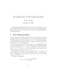
But now, we can reformulate the question about trisection. We can represent
any angle ∠AOB by three points A, O, B. If we restrict ourselves to points from
A, then with the use of the above mentioned coding we obtain the following
new problem: does there exist such Euclid machine that given three numbers
ν(A), ν(O), ν(B), it finds the number representation ν(P ) of the point of the
trisection of ∠AOB, i.e., ∠AOB = 3∠AOP .
The first claim needing justification in this problem is the existence of such
point P with algebraic coordinates. But this fact can be obtained by simple
arithmetic taken from analytic geometry.

B
✬✩
✚ ✚✚✚✚✚ P
O✭✭✭✭✭✭
❤❤❤❤❤❤ A
✫✪
Fig. 3. Angle trisection
Proposition 4.2. For any points A, O, B, with algebraic coordinates, there exists
the point P with algebraic coordinates too, such that ∠AOB = 3∠AOP .
Proof. We use simple methods of analytic geometry to prove that for an angle
placed in the center of a given circle (where the center of this circle and the points
of intersections of the angle with this circle are given by algebraic coordinates),
then the point which gives a solution of the trisection problem on this circle has
also algebraic coordinates.
Without any loss of generality we can identify the point O with the origin
(0, 0), because we can always use a translation with algebraic parameters to
obtain such a situation. Now, we have two lines: OA and OB, for A = (x A , y A ),
B = (x B , y B ) they have the equations: x A y − y A x = 0, x B y − y B x = 0. We can
find now tan(∠AOB) = y Bx A −y A x B
x A x B +y A y B
. Of course, tan( 1 3∠AOB) can be found from
the equation
tan(∠AOB) = 3 tan( 1 3 ∠AOB) − tan3 ( 1 3 ∠AOB)
1 − 3 tan 2 ( 1 3 ∠AOB) ,
which means that tan( 1 3∠AOB) is an algebraic number.
The next step is devoted to compute the coefficient of the line OP given in
the Cartesian plane by y = ax, with a given by
y B
x B
+ tan( 1 3 ∠AOB)
1 − y B
xB
tan( 1 3 ∠AOB)
(x B can always be made different from 0 by some rotation). And now to find
coordinates of P all we need is a solution of the following system of equations
with algebraic coefficients: x 2 P + y2 P = x2 A + y2 A and y P = ax P , such systems have
always algebraic solutions.
□
So, now we are concerned with the crucial question. Can the number ν(P ) be
computed? Our first observation is that if it would be possible for some URM
machine, then this process of computation could be presented in the well known

manner by Euclid machines. By observation of the proof of Proposition 4.2 we
have such the method which can be performed on (possibly infinite) decimal
expansion of the coordinates (for example, by machines of Type Two Theory
[4]). But our problem needs a computation on natural numbers, not on infinite
sequences of digits. And, let us recall, that even if we can generate from the
natural label of some algebraic number x its decimal expansion, it is impossible
to obtain from finite subsequences of this expansion that natural number, which
represents x (from density of the set of algebraic numbers we can always find
infinite number of natural descriptions of algebraic numbers which agree with
given finite sequence of digits).
But the above paragraph does not solve our problem. We can not compute
the ν(P ) from its decimal expansion, but maybe there is some direct method to
solve this problem.
Let us assume at the moment that we have two special families of machines
working on the Euclidean plane possibly with more instructions then Euclid
machines. If we fix some enumeration ν of algebraic points on the Euclidean
plane then for a given pencil of registers described in Section 2.1 we have the
machines E 1 n which for the given X n register with the value k draw the point
P , such that ν(P ) = k. Contrary, the machines E 2 n for given point P draw the
register X n with the value equal to ν(P ).
Theorem 4.1. Let us define the trisection function T : N 3 → N in the following
way
T (ν(A), ν(O), ν(B)) = ν(P ) ⇐⇒ ∠AOB = 3∠AOP.
Moreover, let T ∗ denote the machine working on the Euclidean plane and equivalent
to T . 5 Then the composition of E 1 n ◦ T ∗ ◦ E 2 n is not computable by any
Euclid machine.
Proof. With the above given machines we can draw the trisection in the following
manner. First we translate points A, O, B by E1, 1 E2, 1 E3 1 machines into
X 1 , X 2 , X 3 . Then we use the Euclid version of T to compute ν(P ) in some register,
e.g. X 4 . Then the machine E4 2 draws the solution of the trisection problem.
If this activity could be done with Euclid machines then we would have a contradiction
with Proposition 4.1.
□
We can ask about a possibility of the trisection construction by a ruler and
a compass restricted to points with algebraic coordinates. But, let us recall, the
classical example of impossibility of this construction is the angle of π 3 , which
can be completely described by points with algebraic coordinates.
The above theorem creates a question about a source of Euclid non-computability
of the trisection problem. We have three choices:
1. E 1 n, E 2 n are not Euclid computable, but T is Turing computable;
2. E 1 n, E 2 n are Euclid computable, but T is not Turing computable;
5 T ∗ uses registers in the same way as Euclid machines, but with a possibility of
different instructions.

3. E 1 n, E 2 n are not Euclid computable and T is not Turing computable.
Of course, we know that some points with algebraic coordinates can not
be drawn (with fixed initial points with algebraic coordinates) by a ruler and a
compass. But it is not clear whether this observation implies that E 1 n, E 2 n - which
are some transformations of points on the Euclidean plane - can not be done by
Euclid machines. This consideration leads us to the following conjecture.
Conjecture. If E 1 n, E 2 n are Euclid computable, then T is not Turing computable.
Let us observe that the above statement is always true. But we formulate it
as a conjecture to stress that its non-vacuous character depends on the truth of
the antecedent of the implication, which is still unknown for us.
5 Remarks
It is very interesting to observe that the trisection function does not have a
character of a self-referential problem (like, e.g., the halting problem). It would
be worth of explanation whether such function has any connection to classical
uncomputable functions like the halting function or the busy beaver function.
We can also ask the natural question: is every Euclid computable function
also Turing computable? The obvious suggestion to this question is the answer
YES, by Church’s thesis. Of course, we can interpret this model as a model
with infinite precision, which leads us to comparison with such constructions
as BSS machines. Whatever, the fully mathematical answer will need a precise
construction of a proof.
Let us also add that Fourier series can be interpreted as sums of circles with
decreasing radii. This could be used to obtain another (functional) interpretation
of Euclid machines.
6 Final remark
Part of this work was done ten years ago by Francisco Coelho in collaboration
with José Félix Costa, in the context of his MSc dissertation on Diophantine
equations, advised by Professor Franco de Oliveira from the Universidade de
Évora. Thus we acknowledge Franco de Oliveira as friend and adviser. Let us
also thank to J. F. Costa’s student Bruno Loff and to Udi Boker and Nachum
Dershowitz from Tel Aviv (School of Computer Science) for discussions about
Theorem 8.
References
1. Martin, G.E. Geometric Constructions, Springer-Verlag, 1998.
2. Plouffe, S. The computation of certain numbers using a ruler and compass. Journal
of Integer Sequences, 1, 1998.
3. Shepherdson, J.C. and Sturgis, H.E. Computability of recursive functions. Journal
of the ACM, 10(2), 217-255, 1963.
4. Weihrauch, Klaus. Computable analysis, An Introduction, Springer-Verlag, 2000.