The Size, Structure, and Variability of Late-Type Stars Measured ...
The Size, Structure, and Variability of Late-Type Stars Measured ...
The Size, Structure, and Variability of Late-Type Stars Measured ...

Create successful ePaper yourself
Turn your PDF publications into a flip-book with our unique Google optimized e-Paper software.
<strong>The</strong> <strong>Size</strong>, <strong>Structure</strong>, <strong>and</strong> <strong>Variability</strong> <strong>of</strong> <strong>Late</strong>-<strong>Type</strong> <strong>Stars</strong> <strong>Measured</strong> with<br />
Mid-Infrared Interferometry<br />
by<br />
Jonathon Michael Weiner<br />
B.S. (Michigan State University) 1998<br />
M.A. (UC Berkeley) 2000<br />
A dissertation submitted in partial satisfaction <strong>of</strong> the<br />
requirements for the degree <strong>of</strong><br />
Doctor <strong>of</strong> Philosophy<br />
in<br />
Physics<br />
in the<br />
GRADUATE DIVISION<br />
<strong>of</strong> the<br />
UNIVERSITY <strong>of</strong> CALIFORNIA at BERKELEY<br />
Committee in charge:<br />
Pr<strong>of</strong>essor Charles H. Townes, Chair<br />
Pr<strong>of</strong>essor Sumner P. Davis<br />
Pr<strong>of</strong>essor William J. Welch<br />
2002
<strong>The</strong> <strong>Size</strong>, <strong>Structure</strong>, <strong>and</strong> <strong>Variability</strong> <strong>of</strong> <strong>Late</strong>-<strong>Type</strong> <strong>Stars</strong> <strong>Measured</strong> with<br />
Mid-Infrared Interferometry<br />
Copyright 2002<br />
by<br />
Jonathon Michael Weiner
1<br />
Abstract<br />
<strong>The</strong> <strong>Size</strong>, <strong>Structure</strong>, <strong>and</strong> <strong>Variability</strong> <strong>of</strong> <strong>Late</strong>-<strong>Type</strong> <strong>Stars</strong> <strong>Measured</strong> with Mid-Infrared<br />
Interferometry<br />
by<br />
Jonathon Michael Weiner<br />
Doctor <strong>of</strong> Philosophy in Physics<br />
University <strong>of</strong> California at Berkeley<br />
Pr<strong>of</strong>essor Charles H. Townes, Chair<br />
<strong>The</strong> size <strong>and</strong> variability <strong>of</strong> the photospheres <strong>of</strong> several late-type stars has been probed using<br />
11 µm heterodyne interferometry. High resolution observations performed during the years<br />
1999-2001 yielded diameter measurements accurate to about 1% for a variety <strong>of</strong> stars <strong>of</strong><br />
the supergiant <strong>and</strong> mira variable types. Using narrow b<strong>and</strong>widths (≈ 0.2 cm −1 ) to avoid<br />
spectral lines, visibilities were measured for the stars α Her, χ Cyg, α Ori, o Cet, <strong>and</strong><br />
R Leo. On the latter three stars, observations were made at several different wavelengths,<br />
in some cases overlapping an observed spectral feature. In all cases, the 11 µm sizes are<br />
larger than previously measured visible <strong>and</strong> near-infrared diameters. <strong>The</strong> discrepancies will<br />
be addressed. In addition, a variation <strong>of</strong> the diameter <strong>of</strong> o Cet (Mira) with phase has been<br />
observed.<br />
Pr<strong>of</strong>essor Charles H. Townes<br />
Dissertation Committee Chair
iii<br />
Contents<br />
List <strong>of</strong> Figures<br />
List <strong>of</strong> Tables<br />
v<br />
vii<br />
1 Introduction 1<br />
1.1 Principles <strong>of</strong> Interferometry . . . . . . . . . . . . . . . . . . . . . . . . . . . 2<br />
1.2 History <strong>of</strong> Interferometry . . . . . . . . . . . . . . . . . . . . . . . . . . . . 7<br />
1.3 ISI System . . . . . . . . . . . . . . . . . . . . . . . . . . . . . . . . . . . . 8<br />
1.4 Stellar Evolution <strong>and</strong> AGB <strong>Stars</strong> . . . . . . . . . . . . . . . . . . . . . . . . 11<br />
2 Diameter Measurements Performed with the ISI Compared with Other<br />
Instruments 17<br />
2.1 Diameter Measurements with the ISI . . . . . . . . . . . . . . . . . . . . . . 18<br />
2.2 Comparison <strong>of</strong> ISI Data with Visible <strong>and</strong> Near-IR Measurements . . . . . . 24<br />
2.3 Implications <strong>of</strong> Diameter Measurements . . . . . . . . . . . . . . . . . . . . 28<br />
3 Examination <strong>of</strong> the Accuracy <strong>of</strong> Interferometric Diameter Measurements 31<br />
3.1 Observed Complications to a Straight-Forward Interpretation <strong>of</strong> <strong>Measured</strong><br />
Diameters . . . . . . . . . . . . . . . . . . . . . . . . . . . . . . . . . . . . . 33<br />
3.2 Dust . . . . . . . . . . . . . . . . . . . . . . . . . . . . . . . . . . . . . . . . 34<br />
3.3 Spectral Lines . . . . . . . . . . . . . . . . . . . . . . . . . . . . . . . . . . . 41<br />
3.4 Analysis <strong>of</strong> AGB Atmospheres Including Continuum<br />
Opacity . . . . . . . . . . . . . . . . . . . . . . . . . . . . . . . . . . . . . . 46<br />
3.4.1 Static Radiative Transfer Implied Corrections - Limb Darkening . . 48<br />
3.4.2 <strong>The</strong> Effect <strong>of</strong> Dynamic Phenomena on Stellar Atmospheres . . . . . 52<br />
3.4.3 Cohesive Modelling <strong>of</strong> Stellar Atmospheres <strong>and</strong> 11 µm Diameter Measurements<br />
. . . . . . . . . . . . . . . . . . . . . . . . . . . . . . . . . 58<br />
3.4.4 Investigation <strong>of</strong> Non-LTE Conditions in Atmospheres . . . . . . . . 68<br />
3.5 Explanation <strong>of</strong> Variations in <strong>Measured</strong> Diameter with Wavelength . . . . . 72<br />
4 Time <strong>Variability</strong> in o Cet 77<br />
4.1 Implications <strong>of</strong> Diameter Measurements on Pulsation Mode <strong>and</strong> Dynamics<br />
in Miras . . . . . . . . . . . . . . . . . . . . . . . . . . . . . . . . . . . . . . 78<br />
4.2 Variation <strong>of</strong> the Diameter <strong>of</strong> o Cet with Time . . . . . . . . . . . . . . . . . 79
iv<br />
5 Spectroscopy <strong>and</strong> ISI Measurements <strong>of</strong> Spectral Features 85<br />
5.1 General Results <strong>of</strong> 11 µm Spectroscopy . . . . . . . . . . . . . . . . . . . . 86<br />
5.2 Continuum Measurements at 11.149 µm . . . . . . . . . . . . . . . . . . . . 90<br />
5.3 Modelling Spectral Features in Mira . . . . . . . . . . . . . . . . . . . . . . 96<br />
5.4 Larger <strong>Size</strong>s <strong>Measured</strong> on Spectral Lines . . . . . . . . . . . . . . . . . . . . 101<br />
Bibliography 109
v<br />
List <strong>of</strong> Figures<br />
1.1 Simple Model <strong>of</strong> Interferometer . . . . . . . . . . . . . . . . . . . . . . . . . 3<br />
1.2 Various Examples <strong>of</strong> Visibility Curves . . . . . . . . . . . . . . . . . . . . . 6<br />
1.3 Possible Effective Baseline Coverage for α Ori . . . . . . . . . . . . . . . . . 8<br />
1.4 Simplified Schematic <strong>of</strong> ISI Systems . . . . . . . . . . . . . . . . . . . . . . 10<br />
1.5 Hertzsprung-Russell Diagram <strong>of</strong> ∼9000 <strong>Stars</strong> . . . . . . . . . . . . . . . . . 12<br />
1.6 Stellar Evolution in the H-R diagram . . . . . . . . . . . . . . . . . . . . . . 14<br />
2.1 ISI Data from the night 28Nov00 fit with a uniform disk . . . . . . . . . . . 20<br />
2.2 <strong>The</strong> same ISI Data from 28Nov00 averaged to a fewer number <strong>of</strong> points. . . 20<br />
2.3 Uniform Disk, Limb Darkened Disk, <strong>and</strong> Gaussian Visibility Pr<strong>of</strong>iles Fit to<br />
ISI Data from o Cet on 28Nov00 . . . . . . . . . . . . . . . . . . . . . . . . 22<br />
2.4 Intensity pr<strong>of</strong>iles which correspond to the uniform disk, limb darkened disk,<br />
<strong>and</strong> gaussian visibility curves from Figure 2.3 . . . . . . . . . . . . . . . . . 22<br />
3.1 Absorptivity <strong>of</strong> Silicate Dust vs. Wavelength . . . . . . . . . . . . . . . . . 36<br />
3.2 Intensity Distribution <strong>of</strong> a Star with Dust Shell Forming at 2R ∗ . . . . . . . 38<br />
3.3 Visibilities Corresponding to the Intensity Distribution from Figure 3.2 . . 39<br />
3.4 Apparent Change in Stellar Diameter vs. Dust Formation Radius . . . . . . 40<br />
3.5 Synthetic Near-Infrared Spectra <strong>of</strong> <strong>Stars</strong> at Different Effective Temperatures 42<br />
3.6 Apparent Stellar Diameter vs. Wavelength in the Near-IR . . . . . . . . . . 44<br />
3.7 Predicted CLV <strong>and</strong> Visibility for 1M ⊙ Mira Overtone Pulsator as a Function<br />
<strong>of</strong> Wavelength . . . . . . . . . . . . . . . . . . . . . . . . . . . . . . . . . . . 45<br />
3.8 Ratio <strong>of</strong> Photospheric Diameter to Calculated Uniform Disk Diameter From<br />
Kurucz Model . . . . . . . . . . . . . . . . . . . . . . . . . . . . . . . . . . . 50<br />
3.9 Synthetic Limb Pr<strong>of</strong>iles <strong>of</strong> α Ori from PHOENIX Code . . . . . . . . . . . 51<br />
3.10 Bowen “St<strong>and</strong>ard” Model Density vs. Radius for Different Values <strong>of</strong> Piston<br />
Amplitude . . . . . . . . . . . . . . . . . . . . . . . . . . . . . . . . . . . . . 54<br />
3.11 Predicted Monochromatic Radii vs. Wavelength from Bessell Model . . . . 55<br />
3.12 <strong>Structure</strong> <strong>of</strong> Höfner Long Period Variable Model at Different Phases . . . . 57<br />
3.13 Continuum Opacity <strong>of</strong> <strong>of</strong> Solar Abundance Material at 11.15 µm as a Function<br />
<strong>of</strong> Temperature <strong>and</strong> Density . . . . . . . . . . . . . . . . . . . . . . . . 60<br />
3.14 Dominant Continuum 11.15 µm Opacity Source as a Function <strong>of</strong> Temperature<br />
<strong>and</strong> Density . . . . . . . . . . . . . . . . . . . . . . . . . . . . . . . . . . . . 61
vi<br />
3.15 Density, Temperature, <strong>and</strong> Calculated 11 µm Opacity as a Function <strong>of</strong> Radius<br />
for Static, Radiation Dominated Supergiant Model Atmosphere . . . . . . . 63<br />
3.16 Normalized Synthetic Intensity Pr<strong>of</strong>ile <strong>of</strong> Static Radiation Dominated Supergiant<br />
Model . . . . . . . . . . . . . . . . . . . . . . . . . . . . . . . . . . . . 64<br />
3.17 Density <strong>and</strong> Temperature from Höfner et al. (1998) [47] <strong>and</strong> Calculated 11 µm<br />
LTE Opacity at Maximum (solid line) <strong>and</strong> Minimum (dashed line) Phase . 66<br />
3.18 Normalized Synthetic Intensity Pr<strong>of</strong>ile <strong>of</strong> Höfner et al. (1998) [47] Model at<br />
Maximum <strong>and</strong> Minimum Phase . . . . . . . . . . . . . . . . . . . . . . . . . 67<br />
3.19 Apparent <strong>Size</strong> <strong>of</strong> Höfner Model (Due To Continuum Opacities) at 1.6 <strong>and</strong><br />
11 µm as a Function <strong>of</strong> Phase . . . . . . . . . . . . . . . . . . . . . . . . . . 68<br />
3.20 <strong>The</strong> Temperature, Density, <strong>and</strong> Ionization Fraction in the Wake <strong>of</strong> a Shock<br />
<strong>and</strong> the 11 µm Opacity <strong>and</strong> Integrated Optical Depth <strong>of</strong> the Post-Shock Region 71<br />
3.21 2.1 µm Image <strong>of</strong> 2500 K Star with 3500 K Hotspot <strong>of</strong> Width 0.6R ∗ . . . . . 74<br />
3.22 Visibility Calculated from the Image in Figure 3.21 as a Function <strong>of</strong> the<br />
Magnitude <strong>of</strong> the Spatial Frequency. . . . . . . . . . . . . . . . . . . . . . . 75<br />
4.1 Variation <strong>of</strong> the Diameter <strong>of</strong> o Cet with Phase <strong>and</strong> Date . . . . . . . . . . . 80<br />
4.2 Variation <strong>of</strong> the Diameter <strong>of</strong> α Ori with Date . . . . . . . . . . . . . . . . . 81<br />
4.3 A uniform intensity elliptical star will reproduce the observed 11.1±1.4%<br />
relative size change only if its axial ratio <strong>and</strong> position angle (relative to the<br />
2001 baseline) are within the dashed lines shown above. . . . . . . . . . . . 82<br />
5.1 High Resolution 11 µm Spectra <strong>of</strong> α Ori, o Cet, R Leo, α Her, <strong>and</strong> χ Cyg<strong>and</strong><br />
<strong>The</strong>oretical Water Lines . . . . . . . . . . . . . . . . . . . . . . . . . . . . . 87<br />
5.2 Fractional Absorption or Emission for a Shell <strong>of</strong> Gas . . . . . . . . . . . . . 89<br />
5.3 Best Fitting Calculated Absorption <strong>of</strong> H 2 O vs. Observed Absorption in R Leo 90<br />
5.4 Intensity Pr<strong>of</strong>ile, Implied Visibilities, <strong>and</strong> Best Fit Uniform Disk for Each <strong>of</strong><br />
the Gas Shell Components Presented for o Cet . . . . . . . . . . . . . . . . 91<br />
5.5 Fractional Change in Apparent Diameter Due to a Shell <strong>of</strong> Gas . . . . . . . 93<br />
5.6 Stellar Spectra <strong>of</strong> P20 B<strong>and</strong>pass . . . . . . . . . . . . . . . . . . . . . . . . 95<br />
5.7 Stellar Intensity Pr<strong>of</strong>ile on Spectral Line . . . . . . . . . . . . . . . . . . . . 98<br />
5.8 Model Calculated Spectral Lines . . . . . . . . . . . . . . . . . . . . . . . . 99<br />
5.9 Observed H 2 O Spectral Lines in o Cet . . . . . . . . . . . . . . . . . . . . . 100<br />
5.10 Höfner Model Predicted Spectral Line Pr<strong>of</strong>iles as a Function <strong>of</strong> Phase . . . 102<br />
5.11 o CetVisibilities <strong>and</strong> Best Fitting Uniform Disks from the 11.15 µm Continuum<br />
B<strong>and</strong>pass <strong>and</strong> the 11.086 µm B<strong>and</strong>pass . . . . . . . . . . . . . . . . . . 103<br />
5.12 α Ori <strong>and</strong> R Leo Spectra in Other Observing B<strong>and</strong>passes . . . . . . . . . . 105<br />
5.13 o Cet Spectra in Other Observing B<strong>and</strong>passes . . . . . . . . . . . . . . . . . 106
vii<br />
List <strong>of</strong> Tables<br />
2.1 ISI Diameter Measurements Made in the Years 1999-2001 . . . . . . . . . . 23<br />
2.2 Diameter Measurements from Various Sources: Supergiants . . . . . . . . . 25<br />
2.3 Diameter Measurements from Various Sources: o Cet . . . . . . . . . . . . . 26<br />
2.4 Diameter Measurements from Various Sources: Other Miras . . . . . . . . . 27<br />
2.5 ISI Angular Diameters, Bolometric Fluxes, <strong>and</strong> Implied Effective Temperatures 29<br />
3.1 Possible Continuum Sources <strong>of</strong> Opacity in Stellar Atmospheres . . . . . . . 59<br />
5.1 Increase in Diameter <strong>Measured</strong> in Various B<strong>and</strong>passes Relative to the P20<br />
Continuum B<strong>and</strong>pass . . . . . . . . . . . . . . . . . . . . . . . . . . . . . . . 107<br />
5.2 Höfner Model Predicted <strong>Size</strong> Increase from Observed H 2 O Lines in o Cet in<br />
Various B<strong>and</strong>passes . . . . . . . . . . . . . . . . . . . . . . . . . . . . . . . . 107
viii<br />
Acknowledgements<br />
Over the course <strong>of</strong> my education, a number <strong>of</strong> people have been instrumental in everything<br />
I’ve accomplished. I’d like to thank my parents <strong>and</strong> family <strong>and</strong> Sally for their encouragement.<br />
I want to thank the faculty at Michigan State University, <strong>and</strong> in particular Pr<strong>of</strong>essor<br />
Aaron Galonsky for his advisement during my time there.<br />
It’s been a privilege to work with the past <strong>and</strong> current members <strong>of</strong> the Infrared<br />
Spatial Interferometry group at SSL. I’d like to thank Bill Danchi for teaching me a good<br />
deal about the ISI, Walt Fitelson for his help making it work, Dave Hale for his company<br />
during the observations <strong>and</strong> his knowledge <strong>of</strong> the equipment, <strong>and</strong> Pr<strong>of</strong>essor Charles Townes<br />
for his guidance <strong>and</strong> willingness to help. In addition, John, Peter, Ed, Jeff, Josh, Sam,<br />
Nick, Jerome, Kahina, <strong>and</strong> Jo Ann have all helped me complete this thesis in some way or<br />
another.
1<br />
Chapter 1<br />
Introduction<br />
Astronomy is a peculiar science. Practically everything we’ve learned has come<br />
from the careful study <strong>of</strong> photons coming towards Earth from all directions. But, photons<br />
are slippery as required by the uncertainty relation, <strong>and</strong> to capture one within a telescope<br />
causes it to smear <strong>and</strong> to lose the precise information on from where it came. Of course,<br />
this is diffraction, <strong>and</strong> it places a fundamental limit on the angular resolution a telescope<br />
<strong>of</strong> a given diameter may obtain.<br />
For a conventional telescope, any point on a stellar object will be focused onto the<br />
image plane as a diffraction pattern determined by the size <strong>and</strong> shape <strong>of</strong> the telescope. 1<br />
For a circular aperture telescope, this will be an Airy pattern having full width 2 2.44 λ/D,<br />
where λ is the wavelength <strong>of</strong> the light, <strong>and</strong> D is the diameter <strong>of</strong> the telescope. As a result,<br />
the image is blurred. <strong>The</strong> world’s largest telescope 3 has a limiting aperture <strong>of</strong> 10 m implying<br />
a resolution in blue light <strong>of</strong>:<br />
θ min = 1.22 λ/D = 1.22 × 500 nm/10 m = 6.1 × 10 −8 rad = 12.6 milli − arcseconds<br />
By comparison, the largest stars have apparent angular radii ∼25 milli-arcseconds (mas).<br />
This means stellar structure is unobservable directly, even assuming perfect imaging by<br />
present telescopes.<br />
Fortunately, a solution exists to this problem which does not involve ever larger<br />
telescopes. Interferometry invokes multiple small telescopes positioned at large separations<br />
1 <strong>The</strong> equivalence between diffraction <strong>and</strong> the uncertainty principle applied to photons can be understood<br />
as follows. A photon recorded by a telescope <strong>of</strong> size, D, has uncertainty in position, ∆x ≈ D, implying<br />
∆p x ≥ h/D. But, the uncertainty in the angle, ∆θ = ∆p x/|⃗p| ≥ (h/D)/(hν/c) = λ/D.<br />
2 <strong>The</strong> width is determined by the angle <strong>of</strong> the first zero <strong>of</strong> the Airy pattern intensity.<br />
3 <strong>The</strong> Keck telescope on Mauna Kea is the largest single aperture telescope in the world.
2<br />
to achieve resolution characteristic <strong>of</strong> the separation distance as opposed to the aperture<br />
sizes. <strong>The</strong> coherence <strong>of</strong> the wavefronts emanating from a stellar source are examined to<br />
determine the angular distribution <strong>of</strong> the emitting region. But a h<strong>and</strong>ful <strong>of</strong> separated<br />
apertures can not be exactly equivalent to a single telescope aperature <strong>of</strong> size equal to the<br />
separation. It is partial Fourier coverage <strong>of</strong> the image that is lost. What is meant by this<br />
will be explored in Section 1.1.<br />
This dissertation describes observations <strong>of</strong> evolved red-giant stars using the Infrared<br />
Spatial Interferometer (ISI). <strong>The</strong> observations were performed at 11 µm <strong>and</strong> utilized<br />
baselines long enough to resolve the stellar disk <strong>of</strong> several AGB supergiants <strong>and</strong> Mira variable<br />
stars. <strong>The</strong> thesis contains first a brief introduction into the field <strong>of</strong> interferometry <strong>and</strong><br />
a short discussion <strong>of</strong> stellar evolution <strong>and</strong> AGB stars. Chapter 2 describes the procedure<br />
by which the diameter was calculated from ISI visibility data. Chapter 3 interprets the<br />
diameter measurements within the framework <strong>of</strong> stellar theory <strong>and</strong> compares them with<br />
other observations. Chapter 4 describes the time-like variations seen in the diameter <strong>of</strong><br />
o Cet, <strong>and</strong> Chapter 5 discusses the ISI interferometry performed using a b<strong>and</strong>pass which<br />
contained known spectral lines.<br />
1.1 Principles <strong>of</strong> Interferometry<br />
An interferometer like the ISI can crudely be understood by comparison with<br />
Young’s two-slit experiment. 4 Light from a point source at infinity which takes the form <strong>of</strong><br />
a plane wave passes through the two slits (which represent the two telescope apertures in<br />
an interferometer) <strong>and</strong> forms an interference pattern on the image plane behind the slits.<br />
In this situation, the fringes alternate between total darkness <strong>and</strong> some brightness level,<br />
<strong>and</strong> the visibility, defined by<br />
V = I max − I min<br />
I max + I min<br />
(1.1)<br />
would equal unity since I min = 0. Moreover, this will be independent <strong>of</strong> the separation<br />
<strong>of</strong> the two slits. If another point source is added <strong>of</strong>f from the first by some small angle,<br />
∆θ, it too will form an interference pattern on the image plane, but its pattern will be<br />
shifted due to the slight change in relative path length between the two optical paths. This<br />
scenario is illustrated in Figure 1.1. Because the interference fringes from each <strong>of</strong> the point<br />
4 A more thorough discussion <strong>of</strong> optical interferometry can be found in Born <strong>and</strong> Wolf (1965) [14].
3<br />
Figure 1.1: Simple Model <strong>of</strong> Interferometer for Three Different Telescope Separations. <strong>The</strong><br />
light from each <strong>of</strong> two point sources on an astrophysical object passes through two apertures<br />
as in Young’s double slit experiment <strong>and</strong> each forms an interference pattern on the image<br />
plane behind them. When the two apertures are close together, the interference patterns<br />
are broad <strong>and</strong> their sum adds constructively. As the two apertures are separated, the<br />
interference patterns narrow <strong>and</strong> the sum begins to add destructively.
4<br />
sources are not coaligned perfectly, they will not (necessarily) add constructively. In this<br />
case, the visibility <strong>of</strong> the net fringe pattern may be somewhat less than unity depending<br />
on the separation between the slits. As the slit separation is increased, the visibility falls<br />
<strong>of</strong>f from unity sinusoidally. When the separation between the slits reaches a characteristic<br />
value,<br />
D = λ/2 sin(∆θ) (1.2)<br />
the two interference patterns are completely out <strong>of</strong> phase, the fringes add destructively, <strong>and</strong><br />
the visibility is zero.<br />
This type <strong>of</strong> experiment could be used to measure the angular separation between<br />
the stars in a binary, for instance. An interference pattern could be formed between<br />
two telescopes placed close together. <strong>The</strong>n, the telescopes could be separated until the<br />
fringes disappear. <strong>The</strong> angular separation <strong>of</strong> the two stars would then be given by Equation<br />
1.2. <strong>The</strong> telescopes, separated by a distance, D, could be said to have a resolution,<br />
∆Θ interferometer = λ/2D radians which is similar to the resolution <strong>of</strong> a diffraction limited<br />
single aperture telescope having size on the order <strong>of</strong> the interferometer’s separation as previously<br />
claimed.<br />
For the case <strong>of</strong> an arbitrary intensity distribution, the fringes measured using the<br />
two-slit interferometer will be the superposition <strong>of</strong> all the point source contributions. Since<br />
the net fringes vary sinusoidally with the angular separation between the point sources, the<br />
net fringe can be expressed as an integral over the intensity distribution modulated by a<br />
sinusoidal response. Mathematically, this is equivalent to a two-dimensional Fourier Transform.<br />
This result is known as the Van Cittert-Zernike <strong>The</strong>orem (Born <strong>and</strong> Wolf (1965) [14]),<br />
<strong>and</strong> it states that the complex visibility, V (x, y), is given by,<br />
V (x, y) = 1 F<br />
∫ ∞ ∫ ∞<br />
−∞<br />
−∞<br />
I(θ, φ)e −2πi(θx/λ+φy/λ) dθdφ (1.3)<br />
where [x,y] is the vector baseline (separation) between the two telescopes, F is the total<br />
flux from the source, <strong>and</strong> I(θ, φ) is the intensity distribution on the sky as a function <strong>of</strong> the<br />
angles θ <strong>and</strong> φ (which are assumed to be much less than unity). <strong>The</strong> measured (real-valued)<br />
visibility defined in Equation 1.1 is the magnitude <strong>of</strong> the complex visibility defined above.<br />
To reconstruct an arbitrary intensity distribution from visibility measurements,<br />
one would need to measure the visibility (<strong>and</strong> its phase) on every possible baseline. <strong>The</strong>n,<br />
the image could be reconstructed by inverting Equation 1.3. To accomplish this, one might
5<br />
leave the position <strong>of</strong> one telescope fixed, <strong>and</strong> move the other around to sample as much<br />
<strong>of</strong> the Fourier space as possible. Actually, the rotation <strong>of</strong> the earth changes the effective<br />
baseline throughout the course <strong>of</strong> the night <strong>and</strong> visibility can be recorded along a string <strong>of</strong><br />
baselines without moving either telescope. If the source happens to be circularly symmetric,<br />
as might be expected for spherical objects such as stars, the visibility will also be circularly<br />
symmetric with respect to [x,y], <strong>and</strong> the complex visibility defined in Equation 1.3 will<br />
be real-valued. Thus, the visibility can be considered solely a function <strong>of</strong> the magnitude<br />
<strong>of</strong> the baseline, or <strong>of</strong> the quantity known as spatial frequency which is the magnitude <strong>of</strong><br />
the baseline divided by the wavelength <strong>and</strong> expressed in terms <strong>of</strong> inverse radians. In this<br />
case, the circularly symmetric intensity pr<strong>of</strong>ile <strong>of</strong> the source could be reconstructed from<br />
the fringe visibilities measured on baselines in a single direction.<br />
Figure 1.2 shows some examples <strong>of</strong> circularly symmetric intensity pr<strong>of</strong>iles <strong>and</strong> their<br />
corresponding visibility curves as a function <strong>of</strong> spatial frequency. <strong>The</strong> intensity as a function<br />
<strong>of</strong> radial angle (in milliarcseconds) is plotted on the left with corresponding visibilities to<br />
their right as a function <strong>of</strong> spatial frequency (in 10 5 rad −1 ). It should be noted that to<br />
obtain a visibility curve, it is necessary to take a two-dimensional Fourier Transform <strong>of</strong> the<br />
intensity distribution even if the intensity distribution is circularly symmetric <strong>and</strong> only a<br />
function <strong>of</strong> angular radius. In such a case, the visibility, as a function <strong>of</strong> the magnitude <strong>of</strong><br />
the baseline only, is related to the radial intensity pr<strong>of</strong>ile by a Hankel transform,<br />
V (r) = 1 F<br />
∫ ∞<br />
0<br />
2πθ r dθ r I(θ r )J 0 (2πrθ r /λ) (1.4)<br />
where θ 2 r = θ 2 + φ 2 <strong>and</strong> r 2 = x 2 + y 2 . <strong>The</strong> top two examples in Figure 1.2 illustrate the<br />
Fourier nature <strong>of</strong> interferometry. Wide features in the image are transformed into narrow<br />
features as a function <strong>of</strong> baseline <strong>and</strong> vice-versa. <strong>The</strong> third example is that <strong>of</strong> a uniform<br />
intensity stellar disk. <strong>The</strong> sharp edge to the disk causes “ringing” in the visibility curve.<br />
Most <strong>of</strong> the ISI diameter measurements discussed in Chapter 2 were obtained by fitting<br />
the measured visibility data with the visibility curve corresponding to a uniform disk <strong>of</strong><br />
variable radius. <strong>The</strong> final example in Figure 1.2 illustrates the linear nature <strong>of</strong> the Fourier<br />
transform. <strong>The</strong> visibility curve corresponding to a sum <strong>of</strong> two intensity pr<strong>of</strong>iles is equal to<br />
the sum <strong>of</strong> the visibility curves corresponding to each <strong>of</strong> the pr<strong>of</strong>iles. 5<br />
5 It should be noted that because the visibility curve was defined as normalized to unity at zero spatial<br />
frequency, each component <strong>of</strong> the visibility will be added having a coefficient equal to the fraction <strong>of</strong> the<br />
flux coming from the corresponding component <strong>of</strong> the image.
6<br />
Intensity Pr<strong>of</strong>ile<br />
Hankel Transform<br />
Figure 1.2: Various Examples <strong>of</strong> Visibility Curves. Plotted is the intensity pr<strong>of</strong>ile on the<br />
left (as a function <strong>of</strong> angle), <strong>and</strong> the corresponding visibility curve (as a function <strong>of</strong> spatial<br />
frequency) on the right. <strong>The</strong> top two examples show that wide features on the sky are<br />
transformed into narrow features in Fourier space <strong>and</strong> vice-versa. <strong>The</strong> sharp edge <strong>of</strong> the<br />
uniform disk pr<strong>of</strong>ile is reflected by the “ringing” in the corresponding visibility curve. <strong>The</strong><br />
final pr<strong>of</strong>ile shows that the Fourier Transform is linear <strong>and</strong> that the visibility <strong>of</strong> a sum is<br />
the sum <strong>of</strong> the visibilities.
7<br />
Although a complete set <strong>of</strong> visibility data could be transformed back to the image<br />
domain to obtain the intensity pr<strong>of</strong>ile, this is rarely done. More <strong>of</strong>ten, the coverage <strong>of</strong> the<br />
Fourier domain is too sparse to transform directly <strong>and</strong> is instead analyzed in terms <strong>of</strong> the<br />
limitations it places on the image. For interpretation, a model having a small number <strong>of</strong><br />
variable parameters is usually transformed <strong>and</strong> fit to match the real visibility data. This<br />
extraction <strong>of</strong> real astrophysical information from a set <strong>of</strong> interferometric measurements is a<br />
challenging <strong>and</strong> important part <strong>of</strong> the data reduction process.<br />
1.2 History <strong>of</strong> Interferometry<br />
Using interferometry to obtain higher resolution for astronomical purposes was first<br />
suggested by Fizeau in 1868. <strong>The</strong> first experimental use <strong>of</strong> interferometry on a star was carried<br />
out by Stéphan in 1874 <strong>and</strong> he was unable to resolve any star using his 80 cm reflector<br />
(Quirrenbach (2001) [83]). <strong>The</strong> first measurement <strong>of</strong> the size <strong>of</strong> a star was performed by<br />
Michelson (1921) [70] using a 20 foot baseline within the 100” telescope at Mt. Wilson Observatory.<br />
Betelgeuse (α Ori) was measured to have a diameter <strong>of</strong> 47 mas by Michelson. <strong>The</strong><br />
technologic requirements <strong>of</strong> interferometry did not allow the field to progress after the initial<br />
measurements at Mt. Wilson <strong>and</strong> it wasn’t until the early 1970’s that fringes were formed<br />
from separate telescopes using this type <strong>of</strong> interferometry. This was performed by Labeyrie<br />
in the visible [83], <strong>and</strong> Johnson [53] in the mid-infrared. Since pathlengths in interferometry<br />
need to be matched to within a fraction <strong>of</strong> λ, the strict instrumental requirements <strong>of</strong> optical<br />
interferometry were not present at radio wavelengths. Successful radio interferometers have<br />
been operating since the 1940’s <strong>and</strong> have progressed to the point where intercontinental<br />
baselines are used to obtain resolution competitive with optical instruments. Within the<br />
last 25 years, however, there have been several new optical <strong>and</strong> infrared interferometers<br />
built. Most <strong>of</strong> these are two-telescope arrays using direct fringe detection, although very<br />
recently, several multi-telescope arrays capable <strong>of</strong> phase closure are coming online. <strong>The</strong> current<br />
state <strong>of</strong> optical interferometry is summarized in Quirrenbach (2001) [83] <strong>and</strong> a more<br />
complete history can be found in Shao (1992) [93].
8<br />
Figure 1.3: Possible Effective Baseline Coverage for α Ori Using any Two ISI pads With<br />
α Ori More Than 25 ◦ Above the Horizon<br />
1.3 ISI System<br />
<strong>The</strong> ISI telescope array used to perform the diameter measurements discussed<br />
here is a two-element heterodyne-detection mid-infrared interferometer. <strong>The</strong> ISI consists<br />
<strong>of</strong> two telescopes each having circular apertures 1.65 m in diameter mounted on trailer<br />
frames which allow them to be moved to any <strong>of</strong> a set <strong>of</strong> concrete pads separated by up<br />
to about 72 m. <strong>The</strong> possible effective baseline coverage obtainable using these pads for a<br />
star such as α Ori as it travels from east to west <strong>and</strong> is at least 25 ◦ above the horizon is<br />
illustrated in Figure 1.3. <strong>The</strong> ISI is located at Mt. Wilson Observatory located in the San<br />
Gabriel mountains north <strong>of</strong> Los Angeles, California. <strong>The</strong> site was chosen for its excellent<br />
atmospheric properties. <strong>The</strong> lack <strong>of</strong> fast turbulence above Mt. Wilson causes good “seeing”<br />
in the telescopes <strong>and</strong> is due to relatively low winds <strong>and</strong> a very uniform flow <strong>of</strong> air from
9<br />
the Pacific Ocean nearby. A more complete description <strong>of</strong> the telescopes can be found in<br />
Hale et al. (2000) [37].<br />
<strong>The</strong> interferometer employs heterodyne detection whereby the starlight is mixed<br />
with a CO 2 laser (local oscillator) beam by matching wavefronts <strong>and</strong> focussing both beams<br />
onto a cooled photodiode sensitive to 11 µm radiation. <strong>The</strong> beat signal between the laser<br />
<strong>and</strong> starlight has frequency equal to the difference in their frequencies <strong>and</strong> contains all <strong>of</strong><br />
the phase information from the stellar signal. <strong>The</strong> detector <strong>and</strong> electronics have a passb<strong>and</strong><br />
up to about 3 GHz, so the net b<strong>and</strong>pass used to observe the star lies within the range<br />
[ν LO −3 GHz,ν LO +3 GHz], where ν LO can be chosen to be any <strong>of</strong> a set <strong>of</strong> discrete CO 2 lines<br />
between 9.5 <strong>and</strong> 11.5 µm. <strong>The</strong> two lasers in the telescopes are locked to each other having<br />
a controlled phase difference. After delaying one <strong>of</strong> the beat signals to compensate for the<br />
extra path length to the farthest telescope, the fringe is formed electronically by multiplying<br />
the two beat signals from each telescope. <strong>The</strong> fringe, modulated by the (known) frequency<br />
difference between the lasers, is digitized <strong>and</strong> recorded to disk. A simplified schematic <strong>of</strong><br />
the ISI is shown in Figure 1.4. <strong>The</strong> ISI system is much more complex than described above<br />
<strong>and</strong> a thorough description can be found in Hale et al. (2000) [37].<br />
Heterodyne detection, used by the ISI, can have a better signal to noise ratio than<br />
direct detection (forming fringes directly from starlight) when very narrow b<strong>and</strong>widths are<br />
employed. Additionally, in an interferometric array <strong>of</strong> many telescopes, stellar signals need<br />
to be split into enough beams to form fringes with every other telescope. Using direct<br />
detection, this entails a loss <strong>of</strong> signal to noise. With heterodyne detection, the signals are<br />
electronic radio frequencies <strong>and</strong> can be amplified freely before splitting without losing signal<br />
to noise. A more thorough discussion <strong>of</strong> signal to noise in the ISI compared with direct<br />
detection is found in Monnier (1999) [72] or Hale et al. (2000) [37].<br />
Before 1999, the longest baseline used by the ISI was 30 m. This baseline implies a<br />
resolution typical <strong>of</strong> the circumstellar shells <strong>of</strong> nearby AGB stars. Almost all <strong>of</strong> the science<br />
done with the ISI before 1999 pertained to the structure <strong>of</strong> the dust shells <strong>and</strong> molecular<br />
regions in the circumstellar environment surrounding AGB stars. Much <strong>of</strong> the dust shell<br />
work can be found in Danchi et al. (1994) [22] <strong>and</strong> the interferometry on molecular lines in<br />
Monnier (1999) [72].
10<br />
6LJQDO'HWHFWRU<br />
6LJQDO'HWHFWRU<br />
/DVHU<br />
3KDVH/RFN'HWHFWRU<br />
/DVHU<br />
'HOD\<br />
/LQH<br />
&RUUHODWRU<br />
)ULQJH<br />
Figure 1.4: Simplified Schematic <strong>of</strong> ISI Systems. Starlight collected in each telescope with<br />
the large optics is focussed onto each signal detector along with the beam from a CO 2 laser.<br />
Part <strong>of</strong> the laser beam from telescope #2 is transmitted to telescope #1 where the two<br />
lasers are locked in phase with each other. <strong>The</strong> electronic outputs <strong>of</strong> both signal detectors<br />
are multiplied in the correlator to form the fringe after the signal from telescope #1 is<br />
delayed to compensate for the extra path length to telescope #2.
11<br />
1.4 Stellar Evolution <strong>and</strong> AGB <strong>Stars</strong><br />
<strong>Late</strong>-type AGB stars are ideally suited for observation with the ISI. <strong>The</strong>se stars<br />
are nearing the end <strong>of</strong> their lives, <strong>and</strong> have grown to several hundred times their original<br />
size. Extremely luminous, they have relatively cool temperatures on the order <strong>of</strong> 3000 K.<br />
Because <strong>of</strong> their mostly infrared flux <strong>and</strong> their relatively large angular size, the ISI is able<br />
to obtain accurate visibilities on a number <strong>of</strong> these stars.<br />
<strong>The</strong> following section discusses the stellar life cycle <strong>and</strong>, in particular, the workings<br />
<strong>of</strong> AGB stars like the ones considered within this thesis. It is included to serve as a background<br />
for those unfamiliar with stellar structure <strong>and</strong> evolution <strong>and</strong> to provide a framework<br />
<strong>of</strong> how AGB stars, including the Mira variables <strong>and</strong> supergiants discussed within this thesis,<br />
fit into stellar populations. Most <strong>of</strong> the information pertaining to stellar evolution comes<br />
from Prialnik (2000) [78] <strong>and</strong> Padmanabhan (2001) [74].<br />
A star, by definition, is a gravitationally bound object radiating due to an internal<br />
source. Typically, stars are spherical because gravity acts in a radially symmetric way, <strong>and</strong><br />
their energy source is nuclear fusion occuring in the core. However, energy released from<br />
gravitational self-attraction or stored in the heat capacity <strong>of</strong> its matter is not necessarily<br />
negligible for stellar phenomenon which occur over time scales characteristic <strong>of</strong> these processes.<br />
Although elemental composition does vary between stars, the total stellar mass is<br />
the defining parameter for a star. It determines the size, structure, lifetime, <strong>and</strong> evolutionary<br />
course a star will have. <strong>The</strong> Hertzsprung-Russell (H-R) diagram is a plot <strong>of</strong> the surface<br />
temperature vs. luminosity for a collection <strong>of</strong> stars. Individual stars are points in the plane<br />
<strong>and</strong> variations occur in two dimensions due to the one-parameter variations in both mass<br />
<strong>and</strong> age. Patterns do exist in the H-R diagram, <strong>and</strong> the populations <strong>and</strong> evolutionary tracks<br />
<strong>of</strong> stars within it can be reproduced quite well from theoretical predictions. Figure 1.5 shows<br />
an H-R diagram <strong>of</strong> almost 9000 stars from Perryman et al. (1995) [77]. <strong>The</strong> ordinate <strong>of</strong> the<br />
plot is B-V magnitude instead <strong>of</strong> temperature although these quantities are directly related<br />
for the most part. Only stars whose parallax was measured with precision better than 10%<br />
were plotted. Hence, the collection is not necessarily a representative pool <strong>of</strong> all stars. A<br />
long b<strong>and</strong> <strong>of</strong> stars known as the main sequence is seen to contain most stars. <strong>The</strong>se stars<br />
are in the longest portion <strong>of</strong> their life-cycle <strong>and</strong> vary in mass from about 0.1 M ⊙ at the<br />
bottom-right corner, to 10 M ⊙ in the upper-left. Another grouping <strong>of</strong> stars occurs at higher<br />
luminosities <strong>and</strong> cooler temperatures in the top-right portion <strong>of</strong> the diagram. <strong>The</strong>se are
1995A&A...304...69P<br />
12<br />
Figure 1.5: Hertzsprung-Russell Diagram <strong>of</strong> ∼9000 <strong>Stars</strong> from Perryman et al. (1995) [77].<br />
<strong>The</strong> main-sequence b<strong>and</strong> <strong>of</strong> stars is the dominant shape stretching from high-mass stars<br />
in the top-left to low-mass stars in the lower-right. <strong>The</strong>se stars are in the longest stage <strong>of</strong><br />
their evolution. <strong>Late</strong>-type stars are found above <strong>and</strong> to the right <strong>of</strong> the main-sequence. A<br />
h<strong>and</strong>ful <strong>of</strong> white dwarf stars can be seen in the extreme lower left corner <strong>of</strong> the plot.
13<br />
giant stars nearing the final stages <strong>of</strong> their lives. <strong>The</strong> bottom-left contains a few hot white<br />
dwarf stars which mark the final stage <strong>of</strong> a star’s active life.<br />
<strong>The</strong> stages <strong>of</strong> stellar evolution in the H-R diagram for a star <strong>of</strong> mass 1, 5, <strong>and</strong><br />
25 M ⊙ are outlined in Figure 1.6 (from Iben (1985) [49]). When stars first form from a<br />
collapsing cloud <strong>of</strong> gas, they take their place on the main sequence. Here, hydrogen at<br />
the core is under enough pressure <strong>and</strong> hot enough to fuse. <strong>The</strong> released radiation pressure<br />
supports the star from further gravitational collapse, <strong>and</strong> a steady-state is reached. More<br />
massive stars reach equilibrium at hotter temperatures <strong>and</strong> are more luminous. Most <strong>of</strong> the<br />
life <strong>of</strong> the star is spent on the main-sequence as hydrogen gradually is converted to helium.<br />
More massive stars have much higher rates <strong>of</strong> fusion at their core <strong>and</strong> consequently run out<br />
<strong>of</strong> hydrogen sooner than less massive stars. As the core becomes deficient in hydrogen, the<br />
star enters the next stage in its evolution.<br />
<strong>The</strong> lack <strong>of</strong> hydrogen in the stellar core means much less energy generation at the<br />
star’s center. With no radiation pressure to support it, the core collapses under gravity,<br />
<strong>and</strong> becomes very hot. This causes the hydrogen in the shell surrounding the core to heat<br />
up as well <strong>and</strong> because <strong>of</strong> its extreme temperature dependence, the rate <strong>of</strong> fusion soars.<br />
This radiation increases the luminosity <strong>of</strong> the star several magnitudes, <strong>and</strong> the radiation<br />
pressure causes the outer stellar layers to exp<strong>and</strong> to many times their original size <strong>and</strong><br />
become cooler. As this occurs, the star will move up <strong>and</strong> to the right in the H-R diagram<br />
as shown in Figure 1.6. At this point the star could be classified as a sub-giant. Eventually,<br />
the helium core will become so dense that the degeneracy pressure <strong>of</strong> the free electrons<br />
provide the dominant support against gravitational collapse. When this occurs, the star is<br />
a red giant.<br />
That the star exp<strong>and</strong>s when its core contracts is reproducible using hydrodynamic<br />
theory. However, there is a more fundamental reason that this is so. <strong>The</strong> Virial <strong>The</strong>orem,<br />
applied to a gravitationally bound body composed <strong>of</strong> an ideal gas in hydrostatic equilibrium,<br />
states that the total gravitational potential energy stored in the star is twice the thermal<br />
energy stored in the kinetic motion <strong>of</strong> the gas particles. <strong>The</strong> evolution from main sequence<br />
to giant occurs as the hydrogen in the core is used up. This process occurs slowly enough<br />
that hydrostatic equilibrium can be assumed. <strong>The</strong>rmal equilibrium can also be assumed<br />
if the change in energy <strong>of</strong> the star is small compared to its total energy. In this case, the<br />
Virial theorem will hold. Since the total energy <strong>of</strong> the star is conserved <strong>and</strong> a fixed relation<br />
exists between the thermal <strong>and</strong> gravitational energy, each can be supposed to be conserved
Figure 1.6: Stellar Evolution <strong>of</strong> a 1, 5, <strong>and</strong> 25 M ⊙ Star in the H-R Diagram (reproduction<br />
from Iben (1985) [49]). <strong>The</strong> starting position for the 1, 5, <strong>and</strong> 25 M ⊙ stars lies along the<br />
main-sequence b<strong>and</strong> visible in Figure 1.5 from the top left to the bottom right corner <strong>of</strong> the<br />
H-R diagram. That the star spends most <strong>of</strong> its life in this stage is the reason that most <strong>of</strong><br />
the stars in Figure 1.5 lay along the main-sequence b<strong>and</strong>. As the star evolves, it moves up<br />
<strong>and</strong> to the right in the H-R diagram (towards higher luminosities <strong>and</strong> cooler temperatures).<br />
<strong>The</strong>se later stages <strong>of</strong> stellar evolution are evident as the group <strong>of</strong> stars above <strong>and</strong> to the<br />
right <strong>of</strong> the main sequence in Figure 1.5.<br />
14
15<br />
independently. As a result, a contracting core necessitates an exp<strong>and</strong>ing shell. <strong>The</strong> former<br />
decreases the gravitational potential energy, so in order to maintain gravitational potential<br />
energy conservation the shell must increase its potential energy <strong>and</strong> exp<strong>and</strong>. A similar<br />
process occurs with the temperatures <strong>of</strong> the core <strong>and</strong> the shell. Since thermal energy is<br />
conserved <strong>and</strong> the core heats up, the shell must cool. This trade-<strong>of</strong>f between core <strong>and</strong> shell<br />
properties will continue throughout the star’s life.<br />
As the red giant continues to fuse hydrogen in a shell surrounding the degenerate<br />
core, the helium core grows. During this phase, a large convection zone between the core <strong>and</strong><br />
the stellar surface is formed to transfer the high luminosity outward. This convection mixes<br />
the stars composition <strong>and</strong>, in particular, forces heavier fusion products from the stellar core<br />
to the surface. This is known as “dredge up.” Eventually, if the star has mass greater than<br />
about 0.8M ⊙ , the core reaches a temperature hot enough to fuse helium when its mass<br />
reaches about 0.5M ⊙ . Initially, the extra heat produced by fusing helium doesn’t cause the<br />
core to exp<strong>and</strong> because at this point, it is supported by temperature-independant electron<br />
degeneracy pressure. Consequently, the temperature rises causing the helium fusion rate to<br />
explode. This process happens in a time-scale <strong>of</strong> hours <strong>and</strong> is known as the “helium flash.”<br />
Soon after the helium flash, radiation pressure from the fusing helium causes the<br />
helium core to exp<strong>and</strong> <strong>and</strong> equilibrium is restored. As the core exp<strong>and</strong>s <strong>and</strong> cools, the shell<br />
contracts <strong>and</strong> heats up. This stage, characterized by a core burning helium surrounded by<br />
a shell burning hydrogen, is known as the “helium main-sequence” or “horizontal branch”<br />
<strong>and</strong> it is located below <strong>and</strong> to the left <strong>of</strong> the red giant branch on the H-R diagram, but above<br />
the main sequence. Since there is less helium than there was hydrogen, <strong>and</strong> since helium<br />
burning is about ten times less efficient by mass than hydrogen burning, the helium mainsequence<br />
is much shorter than the first main-sequence. <strong>The</strong> same process which occured<br />
during the main-sequence, a helium core building up, happens again only with the products<br />
<strong>of</strong> helium burning, carbon <strong>and</strong> oxygen, building up in a core. When this core becomes<br />
supported by degeneracy pressure again, the star has reached the asymptotic giant branch<br />
or AGB.<br />
An AGB star is characterized by a very hot <strong>and</strong> dense C/O core supported by<br />
degeneracy pressure. As a result <strong>of</strong> the Virial <strong>The</strong>orem, the outer layers <strong>of</strong> the star exp<strong>and</strong> to<br />
very large sizes <strong>and</strong> extremely cool temperatures. Typical sizes for AGB stars are hundreds<br />
<strong>of</strong> solar radii with surface temperatures as low as 2500 K. As a result, these stars can be<br />
seen in the top-right corner <strong>of</strong> the H-R diagram in Figure 1.5. Many <strong>of</strong> these AGB stars,
16<br />
such as Mira variables, become unstable to pulsation. Dredge-up occurs once more in this<br />
stage <strong>and</strong> carbon <strong>and</strong> oxygen, products <strong>of</strong> helium fusion, become abundant in the stellar<br />
atmosphere. Polyatomic molecules <strong>of</strong> carbon <strong>and</strong> oxygen form in the stellar envelope, <strong>and</strong><br />
solid dust particles form at cooler temperatures further out. <strong>The</strong> greatly extended envelope<br />
implies very low surface gravities allowing radiation pressure to cause some <strong>of</strong> the stellar<br />
mass to become gravitationally unbound from the star. <strong>The</strong> high opacity <strong>of</strong> dust <strong>and</strong><br />
molecules helps drive this process. Mass-loss is observed to be as high as 10 −4 M ⊙ /year in<br />
some AGB stars. It is this assortment <strong>of</strong> characteristics for AGB stars that sets the stage<br />
for the observations described in this thesis.<br />
<strong>The</strong> evolution <strong>of</strong> stars becomes less well known after this stage. Such high rates<br />
<strong>of</strong> mass loss cause the AGB star to break up long before its fuel would have run out.<br />
Eventually, the shell is completely removed <strong>and</strong> only the core remains. <strong>The</strong> star is now a<br />
white dwarf, surrounded by a planetary nebula lit up by hot photons. After ∼ 10 4 years,<br />
the planetary nebula is gone <strong>and</strong> the white dwarf slowly cools for the rest <strong>of</strong> its life. For<br />
high mass stars, elements higher than helium can fuse, <strong>and</strong> the star can end up a neutron<br />
star or black hole, but most <strong>of</strong> the stages <strong>of</strong> its life are analogous.
17<br />
Chapter 2<br />
Diameter Measurements<br />
Performed with the ISI Compared<br />
with Other Instruments<br />
Other than the sun, stars are too small to resolve through st<strong>and</strong>ard single aperture<br />
telescopes 1 . Stellar size is a fundamental property which, for all stars, is accessible only<br />
indirectly, through a h<strong>and</strong>ful <strong>of</strong> techniques.<br />
<strong>The</strong> method <strong>of</strong> lunar occultation involves<br />
recording the light curve <strong>of</strong> a star as it is eclipsed by the moon thus measuring its pr<strong>of</strong>ile.<br />
In aperture synthesis, the aperture <strong>of</strong> an existing large telescope is masked, <strong>and</strong> the fringe<br />
pattern inverted to form an image. It is possible for angular diameters to be crudely derived<br />
through photometry by measuring both the total flux from a star <strong>and</strong> its color temperature.<br />
In at least one case, the limb-darkening <strong>and</strong> size <strong>of</strong> a K-giant was probed through a microlensing<br />
event! (See Albrow et al. (1999) [1].) Finally, interferometry re-constructs the small<br />
angular scale image <strong>of</strong> a star by exploiting the wavelike properties <strong>of</strong> light to achieve a<br />
resolution higher than its component telescopes could obtain alone.<br />
Lunar occultation has been successful at measuring the diameters <strong>of</strong> a number <strong>of</strong><br />
stars. (See White <strong>and</strong> Feierman, 1987 [110].) However, this technique is inherently limited<br />
in its inability to achieve resolution greater than about 1 mas (di Giacomo et al. (1991) [24])<br />
<strong>and</strong> its inflexibility with regard to sky coverage <strong>and</strong> position angle. Aperture synthesis has<br />
provided some <strong>of</strong> the best diameter measurements <strong>of</strong> giant stars at visible <strong>and</strong> near-IR<br />
1 <strong>The</strong> Hubble Space Telescope has reportedly barely resolved the chromosphere <strong>of</strong> α Ori (one <strong>of</strong> the largest<br />
stars) in the ultraviolet. See Gillil<strong>and</strong> <strong>and</strong> Dupree, 1996 [34]
18<br />
wavelengths, however, its range <strong>of</strong> resolution is limited by the size <strong>of</strong> the primary mirror <strong>of</strong><br />
the parent telescope. Photometry is capable <strong>of</strong> very accurate flux measurements at different<br />
wavelengths, but cannot distinguish between effects which would produce similar spectra<br />
while having very different structures. Interferometry is by far the most flexible way <strong>of</strong><br />
measuring the diameters <strong>of</strong> stars. It is not limited to any area <strong>of</strong> the sky, position angle,<br />
range <strong>of</strong> resolution, or wavelength. Thus, it is ideally suited for stellar size measurements.<br />
<strong>The</strong> current technology in interferometry, however, does not yield straight-forward<br />
diameter measurements. In practice, interferometry can measure only a small sample <strong>of</strong> the<br />
available Fourier domain. A direct inversion <strong>of</strong> visibilities to a reasonably complete image<br />
is nearly impossible <strong>and</strong> observations must be compared to a model in order for conclusions<br />
to be drawn. This underscores the importance <strong>of</strong> making diameter measurements at a<br />
wavelength where interpretation is as unambiguous as possible.<br />
2.1 Diameter Measurements with the ISI<br />
<strong>The</strong> stellar diameters obtained with the ISI represent the first 2 measurements <strong>of</strong> a<br />
stellar disk at wavelengths longer than 3 µm. ISI measurements are limited to stars which<br />
are bright enough both at 2 µm <strong>and</strong> at the observing wavelength 3 , <strong>and</strong> are not so obscured<br />
by dust as to block all light from the stellar surface. Also, the angular diameter <strong>of</strong> the<br />
stellar disk must be greater than ≈ 20 mas in order to be well enough resolved for a good<br />
determination <strong>of</strong> its diameter. In practice, we are able to observe late-type stars within<br />
≈ 200 parsecs. In this section, we discuss the diameter measurements <strong>of</strong> the Mira Variable<br />
stars, o Cet, χ Cyg, <strong>and</strong> R Leo, <strong>and</strong> the supergiants, α Ori, <strong>and</strong> α Her.<br />
<strong>The</strong> diameter is obtained from the measured data (visibility squared, V 2 i , with<br />
error, σ V 2<br />
i<br />
, as a function <strong>of</strong> spatial frequency, x i ) by fitting it with the theoretical visibility<br />
function for a disk <strong>of</strong> uniform intensity having a given radius, r. <strong>The</strong>se late-type stars <strong>of</strong>ten<br />
are surrounded by a dust shell at several stellar radii. <strong>The</strong> dust shell is resolved almost<br />
completely at the spatial frequencies we consider (see Section 3.2) so it has the effect <strong>of</strong><br />
lowering the extrapolated visibility at low spatial frequencies by an amount equal to the<br />
fraction <strong>of</strong> light emanating from the extended dust shell.<br />
So, we allow in the fitting, a<br />
2 <strong>The</strong>re have been observations at radio wavelengths with resolutions high enough to resolve stars. <strong>The</strong>y<br />
do not actually “see” the stellar disk at these wavelengths. See Reid <strong>and</strong> Menten, 1997 [84].<br />
3 See Hale et al. (2000) [37] for specific observing requirements including limiting magnitudes, sky coverage,<br />
<strong>and</strong> available b<strong>and</strong>passes.
19<br />
second free parameter, A, to be the fraction <strong>of</strong> light coming from the stellar disk itself. In<br />
this case, the visibity function for the range <strong>of</strong> resolutions reported is given by:<br />
V (x, r, A) = 2AJ 1(2πrx)<br />
2πrx<br />
(2.1)<br />
where x is the spatial frequency in rad −1 , J 1 is the Bessel function <strong>of</strong> order unity, <strong>and</strong> r<br />
is the radius <strong>of</strong> the stellar disk in radians. <strong>The</strong> best-fit radius is given by the minimum <strong>of</strong><br />
χ 2 (r, A) where:<br />
χ 2 (r, A) =<br />
∑ N<br />
i=1 (V 2 (x i , r, A) − V 2<br />
i )2<br />
σ 2 V 2<br />
i<br />
(2.2)<br />
<strong>The</strong> square <strong>of</strong> the visibility was fit as opposed to the visibility because the former is the<br />
directly measured quantity <strong>and</strong> its fluctuations are distributed normally. 4<br />
It should also<br />
be noted that any error in the calibration <strong>of</strong> the visibility data will be absorbed into the<br />
parameter, A, when fit, <strong>and</strong> will not affect the diameter determination.<br />
<strong>The</strong> error in the best-fit stellar disk radius, σ r , was estimated by considering the<br />
region <strong>of</strong> the A-r plane in which the normalized χ 2 is increased by no more than unity<br />
from its minimum. σ r was taken to be one-half the width <strong>of</strong> this region in r. This general<br />
procedure is outlined in Bevington, 1969 [13]. <strong>The</strong> use <strong>of</strong> the normalized χ 2 causes the fit<br />
<strong>of</strong> the stellar radius to have an error which depends only on the spread <strong>of</strong> the data about<br />
the best fit <strong>and</strong> not on the magnitude <strong>of</strong> the σ V 2<br />
i<br />
.<br />
An example <strong>of</strong> a uniform disk fit to a relatively good observing night’s data on<br />
o Cet is shown in Figure 2.1. Figure 2.2 shows the same data averaged so to be clearer<br />
visually. Often, as in this case, a single night <strong>of</strong> observations yields enough data onto which<br />
we can reasonably fit a uniform disk. For weaker stars, or in worse seeing conditions, we<br />
may combine several nights together before fitting. <strong>The</strong>re is rarely a case in which we will<br />
fit data spanning more than a week or so together.<br />
<strong>The</strong> distinction between fitting a uniform disk to the data <strong>and</strong> implying that the<br />
data represents a uniform disk should be noted.<br />
<strong>The</strong> ISI employs effective baselines <strong>of</strong><br />
about 20 - 56 meters. This corresponds to angular resolutions between ∼20 <strong>and</strong> 60 mas.<br />
<strong>The</strong> “sharp” edge <strong>of</strong> a uniform disk pr<strong>of</strong>ile is too narrow a feature to be resolved with the<br />
ISI. <strong>The</strong> correct interpretation <strong>of</strong> our data (as a certain sized disk) is conditional on the<br />
4 At spatial frequencies near the null <strong>of</strong> the visibility function, half <strong>of</strong> the measured data points lie below<br />
zero (because <strong>of</strong> r<strong>and</strong>om fluctuations in the fringe power). <strong>The</strong>ir square roots would not be able to be fitted<br />
to a uniform disk visibility curve.
20<br />
Figure 2.1: ISI Data for o Cet from the night 28Nov00 fit with a uniform disk. <strong>The</strong><br />
starred points represent data taken without chopping for power measurements <strong>and</strong> should<br />
consequently have smaller errors. <strong>The</strong> spatial frequency is expressed in terms <strong>of</strong> spatial<br />
frequency units, or sfu, equal to 10 5 rad −1 . <strong>The</strong> best fit uniform disk has a radius <strong>of</strong><br />
22.97 mas with 25.68% <strong>of</strong> the light coming from the stellar disk. Since the χ 2 <strong>of</strong> the fit<br />
(∼26) is much less than the number <strong>of</strong> data points (65), the model uniform disk is consistent<br />
with the data.<br />
Figure 2.2: <strong>The</strong> same ISI Data from 28Nov00 averaged to a fewer number <strong>of</strong> points. Once<br />
again, χ 2 /N − 2 ≪ 1 indicating a good fit.
21<br />
assumption that the star is a uniform disk. We illustrate this point in Figures 2.3 <strong>and</strong> 2.4.<br />
Figure 2.3 shows the same o Cet ISI data from Figure 2.1 along with a best-fit uniform<br />
disk, limb darkened 5 disk, <strong>and</strong> Gaussian visibility pr<strong>of</strong>ile. It is clear that all three functions<br />
adequately model the observed data. Figure 2.4 shows the three very different intensity<br />
pr<strong>of</strong>iles corresponding to the fits from Figure 2.3. We see that some prior knowledge concerning<br />
the structure <strong>of</strong> the star, (for example, how much limb darkening we may expect),<br />
is quite important if we are to translate the data into useful measurements. <strong>The</strong> size <strong>of</strong><br />
the best-fitting uniform disk is a convenient “diameter” definition for data interpretation,<br />
but it is necessary to relate this measured quantity with theory to extract real information<br />
about the star. <strong>The</strong> theoretical quantity most <strong>of</strong>ten associated with the size <strong>of</strong> a star is the<br />
Rossel<strong>and</strong> diameter. This diameter is defined as twice the radius at which the Rossel<strong>and</strong><br />
opacity 6 equals unity.<br />
<strong>The</strong> ISI diameter measurements made in the years 1999-2001 are displayed in<br />
Table 2.1. All diameters are the result <strong>of</strong> a fit to a uniform disk model. For consistency,<br />
only data with spatial frequency greater than 1.75 × 10 6 rad −1 was used. Each observation<br />
has a b<strong>and</strong>pass centered around the wavelength, λ, with a full width ∼2 nm (or 0.16 cm −1 .)<br />
<strong>The</strong> st<strong>and</strong>ard observation wavelength <strong>of</strong> 11.149 µm was chosen because <strong>of</strong> the relatively<br />
small absorption in Earth’s atmosphere or in the circumstellar material at this wavelength.<br />
<strong>The</strong> other observation wavelengths were chosen in some cases to probe an observed spectral<br />
feature on the star. <strong>The</strong> increased opacity on these molecular lines may cause the star to<br />
appear larger at these wavelengths as evidenced in the table. <strong>The</strong>se spectral measurements<br />
will be discussed in detail in Section 5.4.<br />
It should also be noted that statistically significant changes in the diameters <strong>of</strong><br />
α Ori <strong>and</strong> o Cet were observed over the course <strong>of</strong> several years. <strong>The</strong> fluctuations in α Ori<br />
are relatively small (about 5% in magnitude). By comparison, the size <strong>of</strong> o Cet was seen to<br />
change by more than 18%. <strong>The</strong>se time-like changes will be discussed further in Section 4.2.<br />
5 One parameter power law limb darkening. I(θ) = cos(θ) α where α = 2 in this case <strong>and</strong> θ is the angle<br />
between the line <strong>of</strong> sight <strong>and</strong> the line connecting the center <strong>of</strong> the star to a point on its surface. This<br />
limb-darkening parametrization is discussed in Hestr<strong>of</strong>fer (1997) [42]<br />
6 <strong>The</strong> Rossel<strong>and</strong> opacity is a wavelength averaged opacity weighted towards spectral regions containing<br />
the bulk <strong>of</strong> the emitted flux.
22<br />
Figure 2.3: Uniform Disk, Limb Darkened Disk, <strong>and</strong> Gaussian Visibility Pr<strong>of</strong>iles Fit to ISI<br />
Data from o Cet on 28Nov00<br />
Figure 2.4: Intensity pr<strong>of</strong>iles which correspond to the uniform disk, limb darkened disk, <strong>and</strong><br />
gaussian visibility curves from Figure 2.3
23<br />
Table 2.1: ISI Diameter Measurements Made in the Years 1999-2001: Diameters given are<br />
the results <strong>of</strong> a best-fit to a uniform disk model.<br />
Star Dates Phase λ (µm) Diameter (mas)<br />
α Her 18-31Jul01 11.149 39.32 ± 1.04<br />
α Ori 10-19Nov99 11.149 54.94 ± 0.30<br />
01,08Nov00 11.149 53.42 ± 0.62<br />
28,29Nov00 11.149 55.78 ± 0.92<br />
21Dec00 11.149 54.80 ± 1.00<br />
16-24Aug01 11.149 53.38 ± 0.64<br />
27,28Sep01 11.149 53.28 ± 0.40<br />
04Oct01 11.149 52.56 ± 0.78<br />
11-19Oct01 11.149 53.10 ± 0.52<br />
25,26Oct01 11.086 54.14 ± 0.52<br />
09,16Nov01 11.171 54.20 ± 0.46<br />
19Dec01 11.149 52.66 ± 0.68<br />
χ Cyg 27,30Jul01, 23Aug01 0.51 11.149 39.38 ± 4.02<br />
R Leo 28Oct99 0.43 11.149 55.30 ± 5<br />
19Oct01,02-08Nov01 0.77 11.149 62.62 ± 1.14<br />
09,16Nov01 0.81 11.171 64.24 ± 1.12<br />
o Cet 22,26Oct99 0.99 11.149 46.56 ± 1.43<br />
10-19Nov99 0.06 11.149 49.25 ± 0.55<br />
30Sep00, 03-06Oct00 0.03 11.149 47.63 ± 0.80<br />
17-20Oct00 0.08 11.149 48.84 ± 0.91<br />
01Nov00 0.12 11.149 48.25 ± 0.94<br />
28Nov00 0.20 11.149 47.35 ± 1.24<br />
17,21Dec00 0.27 11.149 46.48 ± 0.84<br />
18-31Jul01 0.92 11.149 50.67 ± 0.63<br />
01-08Aug01 0.95 10.884 57.90 ± 1.52<br />
22,24Aug01 0.01 11.149 53.18 ± 0.67<br />
25-27Sep01 0.11 11.149 53.99 ± 0.53<br />
04,05Oct01 0.13 11.149 51.44 ± 0.67<br />
11Oct01 0.15 11.149 54.27 ± 1.67<br />
23,24Oct01 0.19 11.149 55.06 ± 0.58<br />
25,26Oct01, 02Nov01 0.20 11.086 62.24 ± 0.84<br />
02Nov01 0.22 11.149 52.11 ± 0.95<br />
06-09Nov01 0.24 11.149 52.23 ± 0.50<br />
10-16Nov01 0.26 11.171 55.88 ± 0.74<br />
13,14Dec01 0.35 11.149 49.31 ± 1.04<br />
19Dec01 0.36 11.149 49.92 ± 0.79
24<br />
2.2 Comparison <strong>of</strong> ISI Data with Visible <strong>and</strong> Near-IR Measurements<br />
<strong>The</strong> wide variety <strong>of</strong> techniques <strong>and</strong> instruments capable <strong>of</strong> high resolution studies<br />
have lead to an impressive quantity <strong>of</strong> stellar size measurements. Tables 2.2, 2.3, <strong>and</strong> 2.4<br />
are a compilation <strong>of</strong> some <strong>of</strong> the more recent results for α Ori, α Her, o Cet, χ Cyg, <strong>and</strong><br />
R Leo. <strong>The</strong>se tables list the apparent uniform disk diameter, the observation wavelength,<br />
the technique used to achieve the high angular resolution, the telescope used to make the<br />
observation, <strong>and</strong> in the case <strong>of</strong> the long period variable stars, the variability phase at the<br />
time <strong>of</strong> observation.<br />
Table 2.2 lists the uniform disk diameter <strong>of</strong> two supergiants, α Ori <strong>and</strong> α Her,<br />
measured at different wavelengths. α Ori has been measured extensively, <strong>and</strong> we can instantly<br />
see the difficulty reconciling these measurements. In a few cases, such as the 546 <strong>and</strong><br />
550 nm aperture masking diameters, we observe a discrepancy in measured diameters at<br />
the same wavelength using the same technique. <strong>The</strong>se may result from different b<strong>and</strong>passes<br />
employed, or possibly a time-like change in α Ori between the two measurements. More<br />
generally, we see differences on the order <strong>of</strong> 30% between different wavelengths <strong>of</strong> observation.<br />
<strong>The</strong>se are present even in cases where a single instrument has been used at multiple<br />
frequencies indicating that the discrepancies are probably stellar in origin. <strong>The</strong> general<br />
pattern appears to be large fluctuations in the diameter in the visible, more constant <strong>and</strong><br />
smaller sizes in the near-infrared, <strong>and</strong> larger uniform disk diameters in the mid-infrared.<br />
Although measurements on α Her are less common, the same roughly 20% apparent increase<br />
in size from the K-b<strong>and</strong> (2.2 µm) to mid-infrared is observed. A comprehensive description<br />
<strong>of</strong> these supergiants should account for all <strong>of</strong> the observations. In Chapter 3, we will<br />
attempt to make sense <strong>of</strong> these.<br />
Table 2.3 lists some size measurements for the prototypical Mira variable star,<br />
o Cet. Again, we see large fluctuations in the size <strong>of</strong> Mira with wavelength. We also have<br />
the added possibility <strong>of</strong> variation <strong>of</strong> the diameter with phase since o Cet is a regular variable<br />
star with a period <strong>of</strong> 332 days. Any discrepancies observed at similar wavelengths, (such as<br />
902 <strong>and</strong> 905 nm), are likely explained by the theorized photospheric pulsation occuring in<br />
these stars. <strong>The</strong> apparent size fluctuations for o Cet with wavelength are even larger than<br />
for the supergiants. We see a 200% increase in apparent size from 1.28 to 3.09 µm. <strong>The</strong><br />
mid-infrared ISI continuum measurement at 11.15 µm is about 60% larger than K-b<strong>and</strong>
25<br />
Table 2.2: Diameter Measurements from Various Sources: Supergiants<br />
λ (µm) Diam. (mas) Method ∗ Instrument ref.<br />
α Ori<br />
0.370 52 ± 6 AM KPNO 4m Telescope [20]<br />
0.410 51 ± 2 AM KPNO 4m Telescope [20]<br />
0.520 50 ± 1 AM KPNO 4m Telescope [20]<br />
0.546 57 ± 2 AM Herschel Telescope [111]<br />
0.550 48 ± 1 AM KPNO 4m Telescope [20]<br />
0.633 55 ± 1 AM Herschel Telescope [111]<br />
0.650 58 ± 1 AM KPNO 4m Telescope [20]<br />
0.656 44 ± 1 AM KPNO 4m Telescope [20]<br />
0.700 49 ± 3 AM Herschel Telescope [111]<br />
0.710 54 ± 2 AM Herschel Telescope [111]<br />
0.830 51.1 ± 1.5 I COAST [18]<br />
0.850 46 ± 1 AM KPNO 4m Telescope [20]<br />
0.854 43 ± 1 AM KPNO 4m Telescope [20]<br />
1.09 42 AM Keck Telescope [104]<br />
1.28 42 AM Keck Telescope [104]<br />
1.64 41.5 AM Keck Telescope [104]<br />
2.12 42 AM Keck Telescope [104]<br />
2.2 44.2 ± 0.2 I Michelson Array [26]<br />
3.09 48 AM Keck Telescope [104]<br />
3.75 40.2 ± 0.2 I IOTA [69]<br />
11.09 54.1 ± 0.5 I ISI -<br />
11.15 52.6 - 55.8 I ISI -<br />
11.17 54.2 ± 0.5 I ISI -<br />
several 41.0 ± 0.8 P several [73]<br />
α Her<br />
2.2 32.2 ± 0.8 I Michelson Array [8]<br />
2.2 30.90 ± 0.02 I IOTA [69]<br />
3.75 32.8 ± 0.7 I IOTA [69]<br />
11.15 39.3 ± 1.0 I ISI -<br />
∗ AM: aperture masking, I: interferometry, P: infrared photomotry
26<br />
Table 2.3: Diameter Measurements from Various Sources: o Cet<br />
λ (µm) Phase Diam. (mas) Method ∗ Instrument ref.<br />
o Cet<br />
0.700 0.05-0.58 41 - 44 AM Herschel Telescope [38]<br />
0.710 0.05-0.58 46 - 53 AM Herschel Telescope [38]<br />
0.800 0.96 33 I Mark III [81]<br />
0.800 0.05 26 I Mark III [81]<br />
0.800 0.14 26 I Mark III [81]<br />
0.833 0.05 42.3 ± 3.4 AM Herschel Telescope [38]<br />
0.902 0.05-0.58 36 - 38 AM Herschel Telescope [38]<br />
0.905 0.67 42.0 ± 1.0 ∗∗ I COAST [117]<br />
1.024 0.67 36.3 ± 1.0 ∗∗ I COAST [117]<br />
1.09 0.95 25 AM Keck Telescope [104]<br />
1.290 0.67 31.3 ± 0.5 ∗∗ I COAST [117]<br />
1.28 0.95 20 AM Keck Telescope [104]<br />
1.64 0.95 28.5 AM Keck Telescope [104]<br />
2.12 0.95 34 AM Keck Telescope [104]<br />
2.2 0.94 28.8 ± 0.1 I IOTA [69]<br />
2.2 0.23-0.36 36.1 ± 1.4 I Michelson Array [86]<br />
3.09 0.95 60 AM Keck Telescope [104]<br />
3.75 0.98 43.5 ± 0.2 I IOTA [69]<br />
10.88 0.95 57.9 ± 1.5 I ISI -<br />
11.09 0.20 62.2 ± 0.8 I ISI -<br />
11.15 0.93-1.41 46.5 - 55.1 I ISI -<br />
11.17 0.26 55.9 ± 0.7 I ISI -<br />
several 0.5-1.1 24 - 39 P several [64]<br />
∗ AM: aperture masking, I: interferometry, P: infrared photometry<br />
∗∗ Implied uniform disk diameter. <strong>The</strong> reference listed a Gaussian FWHM which<br />
is a factor <strong>of</strong> ≈ 1.61 times smaller.
27<br />
Table 2.4: Diameter Measurements from Various Sources: Other Miras<br />
λ (µm) Phase Diam. (mas) Method ∗ Instrument ref.<br />
χ Cyg<br />
0.700 0.14-0.35 34 - 44 AM Herschel Telescope [38]<br />
0.710 0.14 41 ± 4 AM Herschel Telescope [38]<br />
0.833 0.32 33 ± 4 AM Herschel Telescope [38]<br />
0.902 0.32 33 ± 2 AM Herschel Telescope [38]<br />
0.905 0.73-1.00 24.7 - 33.6 ∗∗ I COAST [117]<br />
1.024 0.73-1.00 22.3 - 30.7 ∗∗ I COAST [117]<br />
1.290 0.73-1.00 19.5 - 22.4 ∗∗ I COAST [117]<br />
11.15 0.51 39.4 ± 4.0 I ISI -<br />
R Leo<br />
0.650 0.24 67 ± 5 LO Cape, Royal Obs. [110]<br />
0.700 0.88 64.2 ± 5.7 AM Herschel Telescope [38]<br />
0.710 0.88 67.9 ± 7.0 AM Herschel Telescope [38]<br />
0.830 0.05-0.60 38 - 51 I COAST [19]<br />
0.830 0.39-0.60 48 - 51 AM Herschel Telescope [19]<br />
0.833 0.27 44.9 ± 2.0 AM Herschel Telescope [38]<br />
0.902 0.27 43.3 ± 2.0 AM Herschel Telescope [38]<br />
0.940 0.05-0.60 36 - 52 I COAST [19]<br />
0.940 0.39-0.60 47 - 50 AM Herschel Telescope [19]<br />
2.16 0.2 33 ± 1.3 LO TIRGO IR Tel. [24]<br />
2.2 0.24 28.18 ± 0.05 I IOTA [76]<br />
2.2 0.28 30.68 ± 0.05 I IOTA [76]<br />
3.5 0.64 50 LO Hale Observatory [110]<br />
3.75 0.3 44.5 ± 0.2 I IOTA [69]<br />
4.8 0.64 50 LO Hale Observatory [110]<br />
11 0.64 300 LO Hale Observatory [110]<br />
11.15 0.77 62.6 ± 1.1 I ISI -<br />
11.17 0.81 64.2 ± 1.1 I ISI -<br />
∗ AM: aperture masking, I: interferometry, P: infrared photometry, LO: lunar occultation<br />
∗∗ Implied uniform disk diameter. <strong>The</strong> reference listed a Gaussian FWHM which<br />
is a factor <strong>of</strong> ≈ 1.61 times smaller.
28<br />
measurements.<br />
χ Cyg <strong>and</strong> R Leo are also long period variable stars (or Mira variables), <strong>and</strong><br />
Table 2.4 contains recent diameters measured for these stars. Once again, we see large<br />
variations in the apparent size as a function <strong>of</strong> wavelength. For all three Miras, the 710 nm<br />
measurement (which is known to have strong TiO spectral lines) is significantly larger than<br />
the rest. <strong>The</strong> mid-infrared ISI apparent size is again more than 60% larger than nearinfrared<br />
sizes.<br />
2.3 Implications <strong>of</strong> Diameter Measurements<br />
<strong>The</strong> angular diameter <strong>of</strong> a star is an important measured quantity for determining<br />
its structure. When combined with a distance to the star, from an observed parallax for<br />
example, the angular size yields the linear radius. <strong>The</strong> radius sets the length scale for stellar<br />
modelling, <strong>and</strong> is a key component by which our underst<strong>and</strong>ing <strong>of</strong> stellar astrophysics can<br />
be tested. Before Michelson’s first stellar diameter measurement in 1921, it was thought<br />
that all stars were similar to the sun in size, <strong>and</strong> that their angular diameters would be too<br />
small to measure through interferometry. Today, we have a much greater appreciation <strong>of</strong><br />
the roughly 8 orders <strong>of</strong> magnitude by which the size <strong>of</strong> a star may vary. 7 In the case <strong>of</strong> Mira<br />
variables, an accurate diameter will indicate the mode <strong>of</strong> pulsation in the star. <strong>The</strong> pulsation<br />
mode <strong>of</strong> long period variables is a long-st<strong>and</strong>ing subject <strong>of</strong> debate <strong>and</strong> we will return to this<br />
specific question in Section 4.1. <strong>The</strong> linear radius also implies the surface gravity <strong>and</strong> the<br />
average density <strong>of</strong> the star if its mass is known, <strong>and</strong> has important consequences for the<br />
predicted mass-loss occuring in AGB stars <strong>and</strong> the enrichment <strong>of</strong> the inter-stellar medium<br />
through this mechanism. In general, cooler stars are observed to have larger sizes. <strong>The</strong><br />
empirical relationship between angular size, bolometric magnitude, <strong>and</strong> spectral type is<br />
discussed in van Belle, 1999 [106].<br />
<strong>The</strong>re is another parameter which can be directly derived from a star’s angular<br />
diameter, even in the absence <strong>of</strong> knowledge <strong>of</strong> its distance. This is the effective temperature.<br />
It can be determined by knowing only the angular diameter <strong>and</strong> the total flux integrated<br />
over frequency. <strong>The</strong> effective temperature is the temperature, T eff , a spherical black-body<br />
<strong>of</strong> some radius, R, would need to have in order to radiate the given luminosity, L. For this,<br />
7 Neutron stars are thought to have a radius around 30 km. A supergiant such as Betelgeuse has a<br />
measured radius around 5.4 × 10 8 km.
29<br />
we have:<br />
L = 4πR 2 σT 4 eff (2.3)<br />
or, dividing both sides by 4π <strong>and</strong> the square <strong>of</strong> the distance to source, d:<br />
L/(4πd 2 ) = F earth = (R/d) 2 σT 4 eff = θ2 σT 4 eff (2.4)<br />
where F earth is the measured flux on earth, <strong>and</strong> θ is the angular radius obtained through<br />
interferometry or some other technique. Effective temperature is a valuable quantity because<br />
<strong>of</strong> its correspondance with the radiation field energy density. In most stars, convection is the<br />
dominant mechanism for internal energy transport at radii below the stellar surface. Beyond<br />
that, radiation comprises the bulk <strong>of</strong> the transported energy.<br />
In a radiation dominated<br />
atmosphere, the flux through a spherical shell <strong>of</strong> radius, r, is constant with r.<br />
In other<br />
words, the spectral energy distribution may be re-distributed in frequency in a complex<br />
manner due to matter-radiation interactions, but the integrated flux is always fixed. This<br />
makes the emitted flux independent <strong>of</strong> changes in the model atmosphere, <strong>and</strong> quite an<br />
important measured quantity. (See Mihalas, 1978 [71, p. 198–204]) Effective temperature<br />
<strong>and</strong> flux are simply related by F surface = σT 4 eff<br />
provided that the angular radius used to<br />
derive the effective temperature corresponds to the radius at which “most” <strong>of</strong> the photons<br />
were emitted. Thus, an accurate continuum angular diameter along with the total stellar<br />
flux provides a direct <strong>and</strong> unbiased measurement <strong>of</strong> effective temperature <strong>and</strong> the flux in<br />
the outer layers <strong>of</strong> the star.<br />
We can calculate the effective temperatures for α Ori, α Her, o Cet, <strong>and</strong> R Leo, for<br />
which we have measured reasonable diameters. <strong>The</strong>se temperatures are shown in Table 2.5.<br />
<strong>The</strong> table lists the angular diameter measured with the ISI, the frequency integrated bolo-<br />
Table 2.5: ISI Angular Diameters, Bolometric Fluxes, <strong>and</strong> Implied Effective Temperatures<br />
Star Flux (W/m 2 ) ref. Diameter (mas) T eff (K)<br />
α Ori 1.083 × 10 −7 [26] 53.36 3269<br />
α Her 4.09 × 10 −8 [8] 39.32 2986<br />
o Cet(min) 2.128 × 10 −9 [59] 36 ∗ 1490<br />
o Cet(max) 2.668 × 10 −8 [105] 48 2428<br />
R Leo 1.469 × 10 −8 [85] 63.43 1819<br />
∗ This diameter was extrapolated from measurements at other phases
30<br />
metric flux (from the reference cited), <strong>and</strong> the calculated effective temperature. Previously,<br />
Dyck et al. (1992) [26] measured the effective temperature <strong>of</strong> α Ori to be 3520 ± 85 K which<br />
is not too different from our derived value. Our temperature for α Her also is not too different<br />
from Benson et al. (1991) [8] who claimed a value <strong>of</strong> 3210 K. Ridgway et al. (1992) [86]<br />
measured the effective temperature <strong>of</strong> o Cet near maximum to be 2270 ± 140 K, slightly<br />
lower than our value <strong>of</strong> 2428 K. <strong>The</strong> largest discrepancy is between the measurement by<br />
Richichi et al. (1999) [85] <strong>of</strong> 2486 ± 73 K for R Leo compared with our value <strong>of</strong> 1819 K.<br />
<strong>The</strong>se may have been measured at very different phases, however. Richichi et al. (1999) [85]<br />
<strong>and</strong> Perrin et al. (1998) [75] discuss the effective temperatures <strong>of</strong> a moderate sample <strong>of</strong><br />
stars whose diameters have been measured <strong>and</strong> conclusions relating effective temperature<br />
to spectral type are drawn.
31<br />
Chapter 3<br />
Examination <strong>of</strong> the Accuracy <strong>of</strong><br />
Interferometric Diameter<br />
Measurements<br />
<strong>The</strong>re may seem to be little ambiguity in defining the diameter <strong>of</strong> our sun. We<br />
observe the sun to be a bright disk with a well-defined edge which is fairly constant over<br />
visible <strong>and</strong> infrared wavelengths. <strong>The</strong>re would seem to be no more difficulty speaking about<br />
the size <strong>of</strong> our sun than an object like a bowling ball. A closer inspection <strong>of</strong> solar telescope<br />
images would reveal some complications, however. <strong>The</strong> intensity across the stellar surface<br />
is not uniform. It is covered with sunspots which evolve with time. We also observe that<br />
the edges <strong>of</strong> the stellar disk are darker than the center. <strong>The</strong> cooler, outer layers <strong>of</strong> the<br />
photosphere are effectively thicker around the edges due to the spherical geometry <strong>of</strong> the<br />
sun, <strong>and</strong> absorb more light. During an eclipse, we see a corona made up <strong>of</strong> light emanating<br />
from the outer regions <strong>of</strong> the solar atmosphere. So, we concede that, unlike the bowling<br />
ball, the sun does not have a unique radius at which its density falls <strong>of</strong>f to zero.<br />
<strong>The</strong> situation is much more severe when considering late-type AGB stars such<br />
as the supergiants <strong>and</strong> mira variables measured here with the ISI. <strong>The</strong>se stars have radii<br />
several hundred times that <strong>of</strong> the sun with comparable masses in some cases. Thus, their<br />
surface gravities are several orders <strong>of</strong> magnitude lower. This weak gravitational binding is<br />
reflected in the atmospheric extension exhibited by these AGB stars. <strong>The</strong>ir circumstellar<br />
regions contain significant particle densities at radii many times what might be considered
32<br />
their surface. Very <strong>of</strong>ten, material can escape from the gravitational field <strong>of</strong> its parent star<br />
completely <strong>and</strong> mass-loss occurs. We can estimate this effect by considering the hydrostatic<br />
scale height for a stellar atmosphere. A constant temperature gas <strong>of</strong> atomic hydrogen<br />
subject to a gravitational field will have a density which falls <strong>of</strong>f as:<br />
ρ(z) = exp(−m H<br />
gz/kT ) (3.1)<br />
For a star like Mira (with M ≈ 1M ⊙ , R ≈ 700R ⊙ , <strong>and</strong> T ≈ 3000 K), the scale height,<br />
kT/m H<br />
g = 4.7 × 10 10 m, or 0.093 stellar radii. <strong>The</strong> actual density fall-<strong>of</strong>f <strong>of</strong> Mira will be<br />
slower than this due to radiation pressure acting against the gravitational pull, <strong>and</strong> dynamic<br />
shocks which propel material outwards. Hence, the 9.3% extension should serve as a lower<br />
limit. Some structural features, such as dust formation, have been observed at radii several<br />
times the stellar radii.<br />
<strong>The</strong> other defining characteristic for AGB stars is their cool temperatures. Miras<br />
can have surface temperatures as low as perhaps 2500 K. <strong>Stars</strong> having these cool temperatures<br />
radiate a larger fraction <strong>of</strong> their power in the infrared than do sun-like stars. At a<br />
temperature <strong>of</strong> 2500 K, a 1% increase in temperature will result in an increase in blackbody<br />
intensity by 8.24% at 700 nm, 5.79% at 1 µm, 2.83% at 2.2 µm, <strong>and</strong> only 1.28% at<br />
11.149 µm. Hence, at visible <strong>and</strong> near-IR wavelengths the emitted intensity is much more<br />
sensitive to small changes in temperature than at 11 µm. This leads to a less uniform intensity<br />
distribution as observed from earth at these wavelengths. Temperature inhomogeneities<br />
accross the surface <strong>of</strong> AGB stars, possibly arising because <strong>of</strong> turbulence in the convective<br />
region below, will be exaggerated in the visible due to the sensitivity described above <strong>and</strong><br />
the star will appear less like a uniform disk.<br />
Low temperatures in the region surrounding AGB stars have another important<br />
effect concerning the equation <strong>of</strong> state <strong>of</strong> the gases <strong>and</strong> the complicated matter-radiation<br />
interactions occuring just outside the photosphere. Molecules begin to form at temperatures<br />
lower than 3000 K including H 2 , CO, <strong>and</strong> several other oxides <strong>and</strong> carbon molecules. Also,<br />
dust begins to condense at slightly lower temperatures. <strong>The</strong> molecules have many spectral<br />
lines which redistribute the energy distribution <strong>of</strong> the photospheric light. <strong>The</strong> dust scatters<br />
<strong>and</strong> absorbs light, <strong>and</strong> recent model atmosphere calculations have shown that including these<br />
effects can dramatically alter the circumstellar structure. (See Ferguson et al. (2001) [28],<br />
Bowen (1988) [15], <strong>and</strong> Bessel et al. (1996) [10].)
33<br />
3.1 Observed Complications to a Straight-Forward Interpretation<br />
<strong>of</strong> <strong>Measured</strong> Diameters<br />
Within the last decade, departures from uniform disk intensity distributions have<br />
been observed by several high spatial resolution instruments. For several giant stars, including<br />
α Ori, o Cet, <strong>and</strong> R Leo, limb-darkening, hints <strong>of</strong> surface non-uniformity, asymmetries<br />
<strong>and</strong> elongations, <strong>and</strong> time-like changes have been detected at different wavelengths. <strong>The</strong>se<br />
second order corrections to a uniform disk are <strong>of</strong>ten very wavelength dependent <strong>and</strong> could<br />
account for much <strong>of</strong> the discrepancies between diameter measurements at different wavelengths.<br />
A circularly symmetric departure from a uniform disk whereby the intensity falls<br />
<strong>of</strong>f towards the edge <strong>of</strong> the star is known as limb darkening. It occurs when outer, cooler<br />
layers <strong>of</strong> the stellar atmosphere, which are thicker when viewed edge on around the circumference<br />
<strong>of</strong> the star, absorb the hotter continuum photospheric emission. This is reflected<br />
in the image as a more gradual decrease in brightness near the edge <strong>of</strong> the star as compared<br />
to a uniform disk. Some limb darkening has been measured in α Ori at 830 nm<br />
(Burns et al. (1997) [18]), o Cet at 700 nm (Wilson et al. (1992) [111]), α Boo between<br />
450 <strong>and</strong> 800 nm (Quirrenbach et al. (1996) [82]), <strong>and</strong> α Ari <strong>and</strong> α Cas between 520 <strong>and</strong><br />
850 nm (Hajian et al. (1998) [36]). For the α Ori <strong>and</strong> o Cet measurements (Burns et al. <strong>and</strong><br />
Wilson et al. ,) a brightness pr<strong>of</strong>ile having a gaussian-like tail allowed for a much improved<br />
fit with experimental data.<br />
<strong>The</strong>re have been some recent measurements <strong>of</strong> varying surface non-uniformities<br />
on α Ori. Burns et al. (1997) [18] report no asymmetries, <strong>and</strong> no surface features on<br />
α Ori in 1995 contributing more than 4% <strong>of</strong> the total flux at 830 nm. However, Wilson<br />
et al. (1992) [111] observed non-uniformities on α Ori at 546 <strong>and</strong> 710 nm in 1991 <strong>and</strong><br />
Wilson et al. (1997) [112] claimed that at least three bright spots were observed on α Ori<br />
at 700 nm in 1994 totalling more than 20% <strong>of</strong> the flux. Moreover, the positions <strong>of</strong> these<br />
bright spots appeared to change on a weekly time-scale.<br />
Asymmetry <strong>and</strong> elongation in o Cet has also been observed. Karovska et al. (1991)<br />
<strong>and</strong> Karovska et al. (1997) [56, 57] report asymmetries in the visible which vary with wavelength<br />
<strong>and</strong> have axial ratios from 0.77 to 0.93. Wilson et al. (1992) [111] claimed elongation<br />
in o Cet at 700 nm with an axial ratio <strong>of</strong> 0.85. Josselin et al. (2000) [55] observed asymmetries<br />
at somewhat larger radii (∼ 200 mas) in the molecular gas envelope surrounding
34<br />
Mira.<br />
Finally, variations in time <strong>of</strong> stellar features have been seen in several stars from<br />
repeated measurements using a single instrument. Gray (2000) [35] reports non-regular<br />
changes occuring in the spectrum <strong>of</strong> α Ori on time scales ranging from days to years.<br />
Changes in the brightness distribution <strong>of</strong> α Ori over a period <strong>of</strong> 22 months have been observed<br />
by Wilson et al. (1992) [111]. Karovska et al. (1991) [56] have seen changes in the size<br />
<strong>and</strong> asymmetry in o Cet over the course <strong>of</strong> a year. A phase-related change in size by 35% <strong>of</strong><br />
some <strong>of</strong> the atmospheric layers <strong>of</strong> R Leo was reported by Burns et al. (1998) [19]. In contrast,<br />
radio measurements <strong>of</strong> flux density for o Cet <strong>and</strong> R Leo by Reid <strong>and</strong> Menten (1997) [84]<br />
show no variability in the “radio photospheres” <strong>of</strong> these stars (around 2R ∗ ) indicating that<br />
outwardly propagating pulsational disturbances must be damped by some mechanism before<br />
reaching 2R ∗ .<br />
3.2 Dust<br />
<strong>The</strong> cool temperatures <strong>and</strong> relatively high densities in the circumstellar environment<br />
<strong>of</strong> these AGB stars can lead to the precipitation <strong>of</strong> small solids. <strong>The</strong>se sub-micron<br />
sized particles made up <strong>of</strong> carbon or oxides are collectively known as dust. <strong>The</strong> carbon<br />
monoxide molecule, having a strong binding energy, is readily formed in the atmospheres<br />
<strong>of</strong> stars. <strong>The</strong> formation <strong>of</strong> this molecule occurs until almost all <strong>of</strong> the limiting reactant,<br />
carbon or oxygen, is bound. <strong>The</strong> result is that stars with a slight carbon overabundance<br />
end up with no free oxygen in the cool regions <strong>of</strong> its atmosphere, <strong>and</strong> its dust is made up<br />
entirely <strong>of</strong> amorphous carbon particles <strong>and</strong> graphites. Conversely, O-rich stars, such as all<br />
<strong>of</strong> the stars we’re considering, are surrounded by dust shells made up <strong>of</strong> oxides <strong>of</strong> Si, Mg,<br />
Ti, Al, S, Fe, etc.<br />
<strong>The</strong> optical properties <strong>of</strong> the dust are somewhat dependent on the chemistry <strong>and</strong><br />
distribution <strong>of</strong> grain sizes. Measurements <strong>of</strong> laboratory-formed dust have been performed<br />
<strong>and</strong> compared with astronomical data. Martin <strong>and</strong> Rogers (1987) [67] describe some models<br />
for carbon dust compared with spectral observations <strong>of</strong> the carbon star IRC+10216.<br />
Suh (1999) [96] presents the optical properties <strong>of</strong> silicate dust <strong>and</strong> data supporting the<br />
conclusion that silicates are the dominant form <strong>of</strong> dust in O-rich AGB stars. <strong>The</strong> same conclusion<br />
is reached in Danchi et al. (1994) [22] for the five stars considered here. Figure 3.1<br />
reproduces Figure 1 from Suh (1999) [96] comparing the absorptivity <strong>of</strong> 0.1 µm silicate dust
35<br />
from several models. <strong>The</strong> 10 µm feature stems from a resonance <strong>of</strong> the Si–O bond. We<br />
see that the dust is much more opaque in the visible. In addition, there is a great deal <strong>of</strong><br />
scattering that occurs in the visible but not in the mid-infrared due to the characteristic<br />
grain size <strong>of</strong> several hundred nanometers.<br />
We can estimate the structure <strong>of</strong> the dust shell by assuming that the dust particles<br />
are in thermodynamic equilibrium <strong>and</strong> are heated by the central star. In this case:<br />
Radiation Absorbed = Radiation Emitted<br />
L ∗ /4πr 2 = σT 4 (3.2)<br />
Hence, if the temperature at R ∗ is T eff , then<br />
T (r) = T eff (r/R ∗ ) −1/2 (3.3)<br />
Suh (1999) [96] claims silicate dust condenses around 1000 K for the gas densities characteristic<br />
<strong>of</strong> stellar atmospheres. For o Cet, with an effective temperature <strong>of</strong> 2500 K, we estimate<br />
the inner radius <strong>of</strong> dust formation to be 6.25R ∗ . For α Ori, assuming T eff = 3300K, the<br />
radius <strong>of</strong> dust formation is 10.89R ∗ . <strong>The</strong> estimated formation radius for o Cet is very<br />
close to the value <strong>of</strong> 6R ∗ predicted by Lobel et al. (2000) [59] from modelling the spectral<br />
energy distribution <strong>of</strong> Mira. However, it is much larger than the experimentally observed<br />
inner dust shell radius <strong>of</strong> approximately 2R ∗ from Danchi et al. (1994) [22]. For α Ori,<br />
Lobel et al. (2000) [61] estimate the inner radius <strong>of</strong> the dust shell to be ∼ 35R ∗ , whereas<br />
Danchi et al. (1994) [22] measured a thin dust shell to exist at a radius about 40R ∗ surrounding<br />
α Ori. Danchi et al. (1994) [22] also measured inner radii <strong>of</strong> dust formation for<br />
R Leo, χ Cyg, <strong>and</strong> α Her, to be respectively, 1.3 − 2.3R ∗ , 15R ∗ , <strong>and</strong> 12.5R ∗ .<br />
Much <strong>of</strong> the discrepancy between the above dust formation radii values <strong>and</strong> the<br />
simple predictions stems from the variability <strong>of</strong> the stars considered. α Ori is thought<br />
to exhibit non-regular variations <strong>and</strong> there is evidence suggesting that thin dust shells<br />
form at various times <strong>and</strong> are observed exp<strong>and</strong>ing outward in concentric shells (Danchi<br />
et al. (1994) [22]). For o Cet, dynamical models have shown that pulsationally driven<br />
shocks propagating outward through the atmosphere <strong>of</strong> long period variables are followed<br />
by an expansion which cools the gas sufficiently well to cause condensation <strong>of</strong> dust to occur<br />
at much lower radii than would be possible in a static atmosphere (Bowen (1988) [15]). <strong>The</strong><br />
dynamic models <strong>of</strong> Höfner et al. (1998) [47] predict dust formation to occur at radii as low<br />
as 2R ∗ .
36<br />
<br />
<br />
<br />
<br />
<br />
<br />
<br />
<br />
Figure 3.1: Absorptivity <strong>of</strong> Silicate Dust vs. Wavelength for several models (reproduction<br />
<strong>of</strong> Figure 1 from Suh (1999) [96])
37<br />
It has been suggested (Bowen, private communication) that the 11 µm apparent<br />
size <strong>of</strong> a Mira such as o Cet is actually a measure <strong>of</strong> the size <strong>of</strong> an optically thick dust<br />
shell close to (∼1.75 R ∗ ) <strong>and</strong> surrounding the continuum photosphere. In this scenario, the<br />
photospheric radius would be about half the 11 µm apparent size in much closer agreement<br />
with the predictions <strong>of</strong> fundamental mode dynamic pulsation models. (See Section 4.1.)<br />
<strong>The</strong> observed asymmetries <strong>and</strong> elongations in o Cet (See Sections 3.1 <strong>and</strong> 4.2.) also may<br />
be more easily understood if they referred to a close dust shell rather than a photosphere.<br />
However, this possibility can be ruled out by considering the whole <strong>of</strong> observations<br />
<strong>of</strong> o Cet. First, the dust shell would need to be very opaque at 11 µm in order not to allow<br />
any starlight through. Visibilities equalling zero have been recorded with a precision <strong>of</strong><br />
about 1% at spatial frequencies corresponding to the first null <strong>of</strong> the uniform disk implying<br />
an optical depth <strong>of</strong> the hypothetical dust shell significantly greater than unity. <strong>The</strong> opacity<br />
at visible <strong>and</strong> near-infrared wavelengths due to dust absorption is comparable (within an<br />
order <strong>of</strong> magnitude, Figure 3.1) to the 11 µm opacity <strong>and</strong> due to scattering is orders <strong>of</strong><br />
magnitude greater. Hence, some dust would be evident around the smaller stellar disks<br />
observed at these wavelengths. This is not the case. <strong>The</strong> 1.24 µm, 23 mas diameter<br />
measurement <strong>of</strong> o Cet in Tuthill et al. (1999) [104] shows no dust shell contribution to the<br />
flux to an accuracy <strong>of</strong> a few percent.<br />
Finally, the mid-infrared flux is characteristic <strong>of</strong> a hot source, not a cool dust region.<br />
A 12 µm flux <strong>of</strong> 4750 Jy was observed at phase 0.13 on o Cet. (Danchi et al. (1994) [22])<br />
Assuming, as indicated by visibilities, that 25% <strong>of</strong> this flux originates from a region ∼48 mas<br />
in diameter, the emitting region (in LTE) must have an average <strong>of</strong> temperature <strong>of</strong> 2000 K.<br />
Due to the presence <strong>of</strong> a dust shell having optical depth, τ ≈ 0.12 in front <strong>of</strong> the emitting<br />
region, we can estimate its flux to be ∼13% greater, or 5355 Jy, implying a temperature <strong>of</strong><br />
2185 K. This temperature is too hot for dust to exist according to any model. We thus conclude<br />
that the 48 mas feature observed with the ISI is emission from hot gas characteristic<br />
<strong>of</strong> a stellar photosphere <strong>and</strong> not dust.<br />
As explained in Section 2.1, we take into account the dust shell in our uniform<br />
disk fitting by allowing a single free parameter to represent the fraction <strong>of</strong> 11 µm intensity<br />
coming from the dust shell <strong>and</strong> assuming that the dust shell is fully resolved at the lowest<br />
spatial frequencies measured (∼ 20 × 10 5 rad −1 ). This procedure results in no errors if the<br />
dust shell is very large in scale, but could potentially bias diameter measurements if the<br />
dust were not fully resolved at the spatial frequencies used. To estimate how much <strong>of</strong> an
38<br />
Figure 3.2: Intensity Distribution <strong>of</strong> a Star with Dust Shell Forming at 2R ∗<br />
effect a radially symmetric dust shell would have on our diameter fits, we construct a model<br />
dust shell forming at some radius at 1300 K with a temperature distribution proportional<br />
to r −1/2 around a spherical blackbody star <strong>of</strong> temperature 2500 K. (<strong>The</strong> temperature <strong>of</strong><br />
formation <strong>of</strong> 1300 K is somewhat <strong>of</strong> an upper limit <strong>and</strong> would affect the fit more than a<br />
lower value.) We assume the dust is <strong>of</strong> uniform make-up <strong>and</strong> in LTE <strong>and</strong> that there is no<br />
scattering <strong>of</strong> 11 µm light. Finally, we impose a density distribution proportional to r −2<br />
characteristic <strong>of</strong> a uniform outflow. <strong>The</strong> total optical thickness <strong>of</strong> the dust is adjusted so<br />
that a constant 65% <strong>of</strong> the 11 µm radiation emerging is from the dust (based on observed<br />
o Cet visibilities, <strong>and</strong> a decent approximation for the other stars.) Next, we calculate the<br />
intensity distribution for such a model. A plot <strong>of</strong> the emergent intensity distribution for a<br />
star <strong>of</strong> radius 25 mas having a dust shell with radius <strong>of</strong> formation 2R ∗ is shown in Figure 3.2.<br />
<strong>The</strong> sharp peak at 50 mas comes about from viewing the inner edge <strong>of</strong> the dust shell from<br />
the side. A more realistic model would assume that the dust does not form instantaneously,<br />
but the above should serve as a valid approximation. <strong>The</strong> visibilities corresponding to such<br />
an intensity distribution are shown as the individual points in Figure 3.3. <strong>The</strong> uniform
39<br />
Figure 3.3: Visibilities Corresponding to the Intensity Distribution from Figure 3.2 (Individual<br />
Points) <strong>and</strong> the Best Fit Uniform Disk Curve for the Spatial Frequencies Between<br />
20 <strong>and</strong> 45 ×10 5 rad −1 (Solid Line)<br />
disk which best fits these data between 20 <strong>and</strong> 45 ×10 5 rad −1 is plotted as the solid line<br />
in Figure 3.3. In this case, the best fit uniform disk had a radius <strong>of</strong> 24.125 mas (instead<br />
<strong>of</strong> 25 mas) <strong>and</strong> the simulated model visibilities at spatial frequencies greater than 20 × 10 5<br />
rad −1 are almost indistinguishable from that <strong>of</strong> a uniform disk.<br />
This procedure was repeated several times varying the radius <strong>of</strong> formation <strong>and</strong><br />
the best fit uniform disk radius was recorded. <strong>The</strong> relative apparent increase <strong>of</strong> the stellar<br />
diameter as a function <strong>of</strong> dust formation radius is plotted in Figure 3.4. <strong>The</strong> oscillation which<br />
occurs in Figure 3.4 results from the “hard” inner edge to the dust shell. This produces<br />
“ringing” in the visibility with respect to spatial frequency. We see that for stars like α Ori,<br />
α Her, <strong>and</strong> χ Cyg, no correction to the measured diameters will be needed. For o Cet, a<br />
correction <strong>of</strong> +3% ± 1% may be needed if the dust shell measured by Danchi et al. (1994) [22]<br />
is still present. For R Leo, the correction would be +0.8% ± 1% based on the 1.3–2.3 R ∗<br />
dust formation radii given by Danchi et al. (1994) [22]. (Note: to calculate the corrections
40<br />
Figure 3.4: Ratio <strong>of</strong> the Best-Fitting Uniform Disk Diameters <strong>of</strong> the Dust Shell Model to<br />
the Same Model Without Dust<br />
for R Leo, we assumed a stellar diameter <strong>of</strong> 32 mas <strong>and</strong> 45% <strong>of</strong> the 11 µm flux emanating<br />
from the dust corresponding to observed visibilities for R Leo.)<br />
<strong>The</strong> actual dust shells in the stars we’re considering here may, however, be more<br />
complicated. In the very dynamic <strong>and</strong> unstable atmospheres surrounding some AGB stars,<br />
dust formation may not occur spherically symmetrically. Schirrmacher et al. (2001) [88]<br />
describes a mechanism through which small asymmetries in the temperature can be greatly<br />
enhanced by the passage <strong>of</strong> shock waves known to occur in Miras. As the gas cools after<br />
the passage <strong>of</strong> a shock, regions with slightly hotter temperatures are less transparent<br />
than nearby cooler regions, <strong>and</strong> they stay better coupled to the hot radiation field from<br />
the shock, while the cooler regions exp<strong>and</strong> <strong>and</strong> cool efficiently. This phenomenon allows<br />
small inhomogeneities to result in highly asymmetric dust formation in the atmosphere behind<br />
the shock front. Evidence for “clumps” in the dust shell <strong>of</strong> o Cet are presented by<br />
Lopez et al. (1997) [63]. Models including large regions <strong>of</strong> dust with densities ∼ 100 times<br />
the surrounding dust density fit the observations described. <strong>The</strong>re is evidence for asymme-
41<br />
tries in α Ori as well. Lobel <strong>and</strong> Dupree (2001) [62] model the velocity field surrounding<br />
α Ori through spectroscopy. <strong>The</strong>y predict a time-varying asymmetric velocity field containing<br />
at times infalls <strong>of</strong> several km/s on one side <strong>and</strong> outflows on the other. Asymmetries in<br />
the atmosphere <strong>of</strong> α Ori have also been observed by Harper et al. (2001) [39].<br />
We can estimate the effect a clump <strong>of</strong> dust might have on our diameter measurements<br />
by synthesizing visibility measurements from a model having an asymmetric dust<br />
shell, <strong>and</strong> fitting a uniform disk to these data. For the case <strong>of</strong> a small clump <strong>of</strong> dust<br />
(gaussian in shape with a FWHM <strong>of</strong> 15 mas) located at 2R ∗ to the side <strong>of</strong> the star <strong>and</strong><br />
contributing 15% <strong>of</strong> the stellar flux, the apparent diameter will be reduced by 2.2% to 4.1%<br />
depending on the position angle <strong>of</strong> the visibility measurements. If, however, the dust clump<br />
is located at 1R ∗ to the side, or equivalently, in front <strong>of</strong> the star <strong>and</strong> <strong>of</strong>fset from the line <strong>of</strong><br />
sight by 1R ∗ , the apparent diameter will change by -2.6% to +4.1% depending on position<br />
angle. Clumps <strong>of</strong> dust this severe would certainly be observable in the spectrum <strong>of</strong> the<br />
star <strong>and</strong> would lead to stronger than observed non-periodicity in their infrared light curves.<br />
Furthermore, the model from Lopez et al. (1997) [63] which fits 11 µm visibilities contained<br />
an inner clump which contributed only 6% as much flux as the star; about 3 times less than<br />
the model presented above. Hence, we expect any clumping present to be less than the<br />
above estimates.<br />
3.3 Spectral Lines<br />
<strong>The</strong> low effective temperatures <strong>of</strong> AGB stars result in relatively cool circumstellar<br />
material close to the star. In these regions, relatively high densities <strong>and</strong> cool temperatures<br />
induce a variety <strong>of</strong> molecules to form which do not exist around stars like the sun. Some are<br />
simple oxides <strong>and</strong> form in large quantities around O-rich stars, such as CO, TiO, SiO, <strong>and</strong><br />
H 2 O. <strong>The</strong>se di- <strong>and</strong> polyatomic molecules <strong>of</strong>ten have “forests” <strong>of</strong> lines with large wavelengthaveraged<br />
opacities that can significantly affect the emerging spectral energy distribution<br />
(SED) from the star <strong>and</strong> cause dramatic changes in the apparent size <strong>of</strong> the star. <strong>The</strong><br />
redistribution <strong>of</strong> flux due to H 2 O <strong>and</strong> TiO is evident in Figure 3.5 which is a reproduction<br />
<strong>of</strong> Figure 8 from Allard et al. (2000) [3]. <strong>The</strong> plot shows synthetic near-infrared spectra<br />
calculated for a stellar atmosphere for four different values <strong>of</strong> its effective temperature. <strong>The</strong><br />
solid <strong>and</strong> dotted curves stem from using two different lists <strong>of</strong> spectral lines for the H 2 O<br />
transitions. We see that for a 3500 K star, only small amounts <strong>of</strong> the molecules form, <strong>and</strong>
Figure 3.5: Synthetic Near-Infrared Spectra <strong>of</strong> <strong>Stars</strong> at Different Effective Temperatures.<br />
Deep absorption b<strong>and</strong>s due to the line opacity <strong>of</strong> H 2 O <strong>and</strong> TiO are evident. <strong>The</strong> two curves<br />
are from different H 2 O line lists. (reproduction <strong>of</strong> Figure 8 from Allard et al. (2000) [3])<br />
42
43<br />
they form farther out in the atmosphere at lower densities. Thus, the spectrum is rather<br />
clean. Conversely, in the 2000 K star, the water vapor b<strong>and</strong>s are 80–90% deep, indicating<br />
that at these wavelengths, one would observe outer atmospheric layers <strong>of</strong> the star almost<br />
entirely.<br />
<strong>The</strong>re is ample evidence that the spectra <strong>of</strong> real stars, including the AGB stars<br />
considered here, are greatly affected by TiO <strong>and</strong> H 2 O line opacity. (See Tsuji, 2000 [99],<br />
Wing (1997) [113], <strong>and</strong> references therein.) H 2 O lines were observed in α Ori by Jennings<br />
<strong>and</strong> Sada (1998) [52] <strong>and</strong> an H 2 O column density <strong>of</strong> 3 × 10 18 cm −2 was measured.<br />
Tsuji (2001) [100] argues that there exists an observable “warm molecular region” with a<br />
temperature around 1500 K in the atmospheres <strong>of</strong> most or all late-type stars containing<br />
a chemically active soup <strong>of</strong> diatomic <strong>and</strong> polyatomic molecules. <strong>The</strong>re is also significant<br />
evidence to support the claim that the measured sizes <strong>of</strong> stars are affected by the presence <strong>of</strong><br />
molecules. Diameter measurements were made for a number <strong>of</strong> stars with the Mark III interferometer<br />
at both 712 <strong>and</strong> 754 nm. (Quirrenbach et al. , 2001 [79]) <strong>The</strong> 712 nm sizes were<br />
systematically larger, presumably due to the strong TiO b<strong>and</strong>s present at this wavelength.<br />
Moreover, the relative increase in size between the two wavelengths increased for decreasing<br />
effective temperature. <strong>The</strong> effect <strong>of</strong> spectral lines is evident in the stellar diameters <strong>of</strong><br />
Tuthill et al. (1999) [104]. A uniform disk was fit to visibilities taken from Keck telescope<br />
aperture masking at a variety <strong>of</strong> near-IR wavelengths. A reproduction <strong>of</strong> Figure 3 from that<br />
paper showing the best fit diameters vs. wavelength is shown in Figure 3.6. Between 1.3<br />
<strong>and</strong> 3.1 µm, the apparent size <strong>of</strong> α Ori increases from 42 mas to 48 mas, while for o Cet,<br />
it increases from 21 mas to 60 mas! Presumably, this is due to the presence <strong>of</strong> strong TiO<br />
<strong>and</strong> H 2 O b<strong>and</strong>s.<br />
<strong>The</strong> prevalence <strong>of</strong> these polyatomic molecules in AGB stars, <strong>and</strong> the large opacities<br />
<strong>of</strong> their spectral lines may explain many <strong>of</strong> the observed variations in diameter measurements<br />
with wavelength (<strong>and</strong> possibly with time, as well.) Although very model dependent,<br />
variations in the apparent diameters <strong>of</strong> late-type stars in the visible due to TiO are predicted<br />
to be as large as a factor <strong>of</strong> 2.5 (see Jacob et al. , 2000 [50]). In most cases, the extra<br />
opacity at radii greater than the photosphere’s produces extension in the stellar pr<strong>of</strong>ile <strong>and</strong><br />
a larger diameter would be measured such as is shown in the measurements <strong>of</strong> Quirrenbach<br />
et al. (2001) [79]. In some cases, the line can darken the star around its edges <strong>and</strong> a<br />
smaller value for its radius can be recorded. This “extreme limb-darkening” is discussed in<br />
H<strong>of</strong>mann et al. (1998) [46] <strong>and</strong> for some Mira models can result in a factor <strong>of</strong> ∼2 smaller
44<br />
Angular Diameter (mas)<br />
60<br />
50<br />
40<br />
30<br />
20<br />
10<br />
Stellar Diameter vs. Wavelength<br />
W Hya<br />
Alp Tau<br />
Alp Ori<br />
o Cet<br />
0<br />
1.0 1.5 2.0 2.5 3.0<br />
Wavelength (µm)<br />
Figure 3.6: Apparent Stellar Diameter vs. Wavelength in the Near-IR for the stars W Hya,<br />
α Tau, α Ori, <strong>and</strong> o Cet. <strong>The</strong> effect <strong>of</strong> strong TiO <strong>and</strong> H 2 O b<strong>and</strong>s are evident. (reproduction<br />
<strong>of</strong> Figure 3 from Tuthill et al. (1999) [104])<br />
uniform disk radii at strong TiO absorption b<strong>and</strong>s (such as 710 nm) as compared to nearinfrared<br />
continuum radii. <strong>The</strong>se two opposing theoretically predicted effects are illustrated<br />
in Figure 3.7 which is a reproduction <strong>of</strong> Figure 6 from Jacob et al. (2000) [50]. <strong>The</strong> plots are<br />
the results <strong>of</strong> a 1M ⊙ mira overtone pulsator model, as it would appear at different wavelengths.<br />
<strong>The</strong> top plot shows the radii at which the intensity falls to 90, 50, 10, <strong>and</strong> 2% <strong>of</strong> its<br />
peak value. <strong>The</strong> middle shows the calculated visibility at 1, 2, <strong>and</strong> 3 × 10 6 rad −1 , <strong>and</strong> the<br />
bottom shows the synthesized spectrum <strong>and</strong> a magnification <strong>of</strong> itself. <strong>The</strong> dotted vertical<br />
lines roughly mark the centers <strong>of</strong> the TiO absorption b<strong>and</strong>s in the spectrum. We see that<br />
at strong TiO b<strong>and</strong>s in the visible, the intensity radii are reduced <strong>and</strong> the visibilities increased<br />
causing the fit diameter to be smaller than in the continuum surrounding the b<strong>and</strong>.<br />
However, in the near-IR, the opposite effect occurs. <strong>The</strong> 930 <strong>and</strong> 1060 nm TiO b<strong>and</strong>s cause<br />
the intensity to fall <strong>of</strong>f at larger radii <strong>and</strong> have lower visibilities than at adjacent continuum
45<br />
Figure 3.7: Predicted CLV <strong>and</strong> Visibility for 1M ⊙ Mira Overtone Pulsator as a Function<br />
<strong>of</strong> Wavelength. Top: Radii at which intensity drops to 90, 50, 10, <strong>and</strong> 2% <strong>of</strong> its peak value.<br />
Middle: Visibility at 1, 2, <strong>and</strong> 3 × 10 6 rad −1 . Bottom: Synthetic model spectrum <strong>and</strong><br />
20× magnification all plotted against wavelength in the visible/near-IR (reproduction <strong>of</strong><br />
Figure 6 from Jacob et al. (2000) [50])
46<br />
wavelengths which would cause the diameter measurement to be larger than in the continuum.<br />
It should be noted that other mira atmospheric models in Jacob et al. (2000) [50]<br />
result in characteristic increases in apparent size in all <strong>of</strong> the TiO b<strong>and</strong>s modelled. <strong>The</strong><br />
possibility <strong>of</strong> spectral opacity causing increases or decreases in the apparent size <strong>of</strong> the star<br />
is also exhibited by the simple thin shell models considered in Section 5.2.<br />
<strong>The</strong> importance <strong>of</strong> unbiased continuum diameters makes avoiding spectral lines in<br />
stellar size measurements quite valuable. This can be accomplished by choosing spectral<br />
b<strong>and</strong>s which do not contain significant absorption. <strong>The</strong> use <strong>of</strong> narrow b<strong>and</strong>passes facilitates<br />
extracting continuum diameter measurements provided that a high resolution spectrum can<br />
be used to choose an observing region free <strong>of</strong> spectral contamination. Wide b<strong>and</strong>widths, on<br />
the other h<strong>and</strong>, effectively average over wavelength <strong>and</strong> are incapable <strong>of</strong> separating out the<br />
effect <strong>of</strong> lines which may be present.<br />
<strong>The</strong> ISI uses an assortment <strong>of</strong> narrow (∼0.17 cm −1 ) b<strong>and</strong>passes <strong>and</strong> through the<br />
use <strong>of</strong> high resolution spectra obtained with the IRTF telescope can select line-free observing<br />
regions in which to make continuum diameter measurements. <strong>The</strong> detailed analysis <strong>of</strong> the<br />
11 µm spectra <strong>and</strong> the possible effects <strong>of</strong> spectral contamination on ISI observations are<br />
discussed in Sections 5.1 <strong>and</strong> 5.2. Considerations based on known H 2 O spectral lines within<br />
the chosen ISI observing b<strong>and</strong>pass imply only a small correction to our measured diameters<br />
<strong>of</strong> between 0.0% <strong>and</strong> +0.2%. <strong>The</strong> effect <strong>of</strong> spectral contamination due to gases other than<br />
H 2 O is more uncertain, but should be no more than 1% for the 11.149 µm b<strong>and</strong>pass for any<br />
<strong>of</strong> the stars.<br />
3.4 Analysis <strong>of</strong> AGB Atmospheres Including Continuum<br />
Opacity<br />
In order to fully underst<strong>and</strong> the variety <strong>of</strong> interferometric measurements obtained<br />
for AGB stars, it is necessary to construct a model complete enough to explain the observations.<br />
Such a model should contain adequate descriptions <strong>of</strong> the dust formation <strong>and</strong><br />
molecular line opacities as it was shown previously that these result in important modifications<br />
to the intensity distribution emerging from the star at some wavelengths. However,<br />
there are limits to treating the photosphere itself as a spherical blackbody. A physical star<br />
has no discontinuity in its density as a function <strong>of</strong> radius. Rather, the density <strong>and</strong> temper-
47<br />
ature fall <strong>of</strong>f continuously in the circumstellar regions. Consequently, the optical depth can<br />
be very wavelength dependent <strong>and</strong> some spectral regions may see much larger continuum<br />
photospheres than others. High resolution studies performed at radio <strong>and</strong> ultraviolet frequencies<br />
have measured continuum radii more than twice as large as visible continuum radii<br />
for some AGB stars. (Gillil<strong>and</strong> <strong>and</strong> Dupree (1996) [34] <strong>and</strong> Reid <strong>and</strong> Menten (1997) [84])<br />
A comprehensive explanation <strong>of</strong> the data can be had by solving the radiative transfer problem<br />
<strong>and</strong> obtaining the state <strong>of</strong> the gas everywhere around the star. A prediction <strong>of</strong> what<br />
would be seen at any given wavelength could then be made. In practice, there are many<br />
complications to such an idealized procedure.<br />
For low effective temperature stars, the equation <strong>of</strong> state <strong>of</strong> the circumstellar<br />
material can be very complicated. For instance the presence <strong>of</strong> molecules in the atmospheres<br />
<strong>of</strong> stars can depend very sensitively on relative abundances <strong>of</strong> the chemical elements in the<br />
parent star. <strong>The</strong>se molecules, through their line opacity, can couple efficiently the radiation<br />
pressure from the star to the (what would have been) transparent gases. Winds may<br />
be formed <strong>and</strong> the extension <strong>of</strong> the stellar atmosphere increased significantly relative to<br />
hydrodynamic equilibrium. This may result in more or different molecules or dust forming<br />
<strong>and</strong> altering the star further. (Helling et al. (2000) [41]) In this way, small changes in<br />
the initial stellar composition or luminosity may induce pr<strong>of</strong>ound changes in its observable<br />
properties.<br />
Breaking <strong>of</strong> the spherical symmetry <strong>of</strong> a star may also occur in the outer regions<br />
<strong>of</strong> its photosphere. Large convective cells may cause hotspots on the stellar surface capable<br />
<strong>of</strong> lessening the apparent size <strong>of</strong> the star. (Predicted by Schwarschild (1975) [91] <strong>and</strong><br />
possibly observed in α Ori by Dupree <strong>and</strong> Gillil<strong>and</strong> (1995) [25]) Other asymmetries may<br />
be caused by non-radial pulsational modes in Miras. <strong>The</strong> beginnings <strong>of</strong> a bi-polar planetary<br />
nebula have even been suggested as the cause <strong>of</strong> an observed elongation in o Cet by<br />
Josselin et al. (2000) [55].<br />
Finally, the Miras <strong>and</strong> α Ori are known to exhibit dramatic temporal changes<br />
in their luminosities. Changes at visible wavelengths <strong>of</strong> several magnitudes are common<br />
for Miras. Strong shock waves also are observed in their line pr<strong>of</strong>iles. <strong>The</strong> complicated<br />
dynamics <strong>of</strong> these large stars further obscures their properties. Pulsationally driven stellar<br />
atmosphere models have progressed; however, no current model is capable <strong>of</strong> including<br />
any but the simplest frequency dependence to the radiation field, much less non-spherical<br />
dynamics. In the following sections we will attempt to address all <strong>of</strong> these concerns.
48<br />
3.4.1 Static Radiative Transfer Implied Corrections - Limb Darkening<br />
A spherically symmetric atmosphere characterized by a balance <strong>of</strong> radiation pressure<br />
<strong>and</strong> hydrostatic forces can be modelled through consideration <strong>of</strong> the photon-matter<br />
interactions. Essentially, a stable solution would consist <strong>of</strong> knowing the state <strong>of</strong> the gas as<br />
a function <strong>of</strong> radius (which may or may not be in thermodynamic equilibrium), <strong>and</strong> the<br />
full wavelength dependent radiation field. For a steady state to occur, the radiation given<br />
<strong>of</strong>f by the stellar interior must interact with each shell <strong>of</strong> atmosphere (through absorption,<br />
emission, or scattering by its constituents) in such a way as not to change its state (including<br />
kinetic temperature, excitational levels, <strong>and</strong> degrees <strong>of</strong> molecular dissociation <strong>and</strong><br />
ionization.) Such a model involves detailed underst<strong>and</strong>ing <strong>of</strong> the microphysics, including a<br />
complete list <strong>of</strong> spectral lines for all species involved. Modern computing, using millions <strong>of</strong><br />
atomic <strong>and</strong> molecular transitions, has refined the process a great deal.<br />
<strong>The</strong>oretically, the model-calculated emergent intensity distribution could be inverted<br />
to a visibility pr<strong>of</strong>ile <strong>and</strong> compared directly to interferometric observations. In practice,<br />
a model will generally be fit with a uniform disk function, <strong>and</strong> this quantity, as a<br />
function <strong>of</strong> wavelength, will be compared with observations. A static model atmosphere<br />
has obvious limitations, but should reproduce observations for non-variable supergiants<br />
well. A semi-regular variable, such as α Ori or α Her, may exhibit some phenomenon not<br />
included in a static model, <strong>and</strong> the applicability <strong>of</strong> these results to Mira variables is even<br />
more questionable.<br />
<strong>The</strong> pr<strong>of</strong>iles <strong>of</strong> late-type giant stars were calculated using a plane-parallel approximation<br />
in the visible by M<strong>and</strong>uca et al. (1977) [66] <strong>and</strong> extended to the infrared by<br />
M<strong>and</strong>uca (1978) [65]. <strong>The</strong> model atmospheres were calculated as a function <strong>of</strong> effective<br />
temperature, metallicity, surface gravity, <strong>and</strong> wavelength between ∼400 nm <strong>and</strong> 5 µm. <strong>The</strong><br />
lowest effective temperature model was 3750 K with a surface gravity <strong>of</strong> 31.6 cm/s 2 . By<br />
comparison, a 15M ⊙ star at 131 pc with a diameter <strong>of</strong> 50 mas (similar to α Ori) would<br />
have a smaller surface gravity <strong>of</strong> 0.83 cm/s 2 while a 1M ⊙ star at 117 pc with a diameter <strong>of</strong><br />
39 mas (similar to α Her) would have a surface gravity <strong>of</strong> 0.11 cm/s 2 . <strong>The</strong> M<strong>and</strong>uca model<br />
atmosphere produces limb darkening which reduces the observable diameter monotonically<br />
with decreasing wavelength. At 700 nm, the predicted apparent size <strong>of</strong> the star is reduced<br />
by 9.50%, whereas, at 5 µm, it is reduced by only 2.09%. <strong>The</strong> basic cause <strong>of</strong> the reduction<br />
in limb darkening in the infrared stems from the relative insensitivity <strong>of</strong> intensity on
49<br />
temperature at these wavelengths <strong>and</strong> the lessening <strong>of</strong> extra-photospheric opacity.<br />
<strong>The</strong> atmospheres <strong>of</strong> M-supergiants, including effective temperatures as low as<br />
2500 K, were modelled by Scholz <strong>and</strong> Takeda (1987) [89] <strong>and</strong> further by H<strong>of</strong>mann <strong>and</strong><br />
Scholz (1998) [45]. <strong>The</strong> latter calculated the uniform disk diameters best fitting the model<br />
center to limb variation (CLV). For an α Her-like star, with an effective temperature <strong>of</strong><br />
3000 K <strong>and</strong> luminosity <strong>of</strong> 10 4 L ⊙ , the uniform disk diameter generally becomes less limb<br />
darkened with increasing wavelength. <strong>The</strong> visible region exhibits uniform disk sizes larger<br />
than the Rossel<strong>and</strong> radii with very non-uniform pr<strong>of</strong>iles due to TiO opacity at large radii,<br />
while the near-infrared exhibits some limb darkening causing a shrinkage in the best fit<br />
uniform disk diameter. <strong>The</strong> magnitude <strong>of</strong> the change in apparent size ranges from -5% at<br />
400 nm to +21% at 710 nm to -4% at 1.04 µm to 0% at 3.8 µm. <strong>The</strong> calculation does not<br />
include wavelengths longer than 3.8 µm.<br />
Jacob <strong>and</strong> Scholz (2002) [51] discuss the model predicted effects <strong>of</strong> molecular line<br />
contamination on diameters <strong>of</strong> Mira stars measured with interferometry. <strong>The</strong> paper concludes<br />
that the uniform disk diameters obtained by fitting visibilities can be very dependent<br />
on phase, cycle, <strong>and</strong> even baseline (since the CLV may be very different from a uniform<br />
disk). All <strong>of</strong> the b<strong>and</strong>passes considered were near-IR <strong>and</strong> broad in wavelength coverage,<br />
not allowing for the total exclusion <strong>of</strong> spectral lines. In the b<strong>and</strong>passes most affected by<br />
lines, the models predict interferometrically derived diameters to be more than a factor <strong>of</strong><br />
two larger than Rossel<strong>and</strong> or monochromatic diameters.<br />
Davis et al. (2000) [23] calculate the limb darkening corrections for uniform disk<br />
diameter measurements based on the Kurucz model stellar atmospheres assuming compact<br />
photospheres for effective temperatures as low as 3500 K with surface gravities <strong>of</strong> 10 4 cm/s 2<br />
(typical <strong>of</strong> main-sequence stars). Although not strictly applicable to extended late-type<br />
giants, the calculations extend to 10 µm in wavelength. <strong>The</strong> ratio <strong>of</strong> the photospheric<br />
diameter to the measured uniform disk diameter, ρ θ , is plotted against wavelength for<br />
a variety <strong>of</strong> model parameters in Figure 3.8 which is a reproduction <strong>of</strong> Figure 1 from<br />
Davis et al. (2000) [23]. We see that the effect becomes less than 1% at 10 µm, for each <strong>of</strong><br />
the models shown here.<br />
<strong>The</strong> PHOENIX model atmosphere code was used to simulate the atmosphere <strong>of</strong><br />
α Ori <strong>and</strong> calculate the expected CLV at both 2.25 µm <strong>and</strong> 11.15 µm where visibility<br />
measurements have been made. 1 <strong>The</strong> best fitting uniform disk for α Ori at 2.25 µm has<br />
1 <strong>The</strong> 2.25 µm visibilities were obtained through aperture masking <strong>of</strong> the Keck Telescope as described in
50<br />
Figure 3.8: Ratio <strong>of</strong> Photospheric Diameter to Limb Darkened Disk Diameter From Kurucz<br />
Model Atmospheres as a Function <strong>of</strong> Wavelength. <strong>The</strong> models have solar abundances <strong>and</strong><br />
various surface gravities <strong>and</strong> effective temperatures. (a) T eff = 3500 K, log g = 4.5, (b)<br />
T eff = 5500 K, log g = 4.5, (c) T eff = 10000 K, log g = 4, (d) T eff = 15000 K, log g = 4, (e)<br />
T eff = 20000 K, log g = 4. (reproduction <strong>of</strong> Figure 1 from Davis et al. (2000) [23])<br />
a diameter <strong>of</strong> 42 mas, whereas the 11.15 µm diameter is 54 mas, a 29% difference. <strong>The</strong><br />
PHOENIX code uses a spherical (as opposed to plane parallel) radiative transfer <strong>and</strong> a<br />
molecular line list containing 5×10 8 transitions. It is outlined in Hauschildt et al. (1999) [40].<br />
Model predicted CLVs <strong>of</strong> giant stars are discussed in Aufdenberg <strong>and</strong> Hauschildt (2002) [6]’.<br />
An effective temperature <strong>of</strong> 3500 K <strong>and</strong> a surface gravity <strong>of</strong> 0.316 cm/sec 2 was chosen<br />
to model α Ori, <strong>and</strong> the mass was varied. <strong>The</strong> synthetic limb pr<strong>of</strong>ile for an 8M ⊙ <strong>and</strong><br />
0.5M ⊙ star as it would appear in each <strong>of</strong> the two b<strong>and</strong>passes described above is shown<br />
in Figure 3.9. <strong>The</strong>se were obtained from J. P. Aufdenberg <strong>and</strong> P. H. Hauschildt through<br />
Tuthill et al. (1999) [104].
51<br />
Figure 3.9: Synthetic Limb Pr<strong>of</strong>ile from PHOENIX Code for an 8M ⊙ <strong>and</strong> 0.5M ⊙ star at<br />
2.25 <strong>and</strong> 11.15 µm. (from J. P. Aufdenberg <strong>and</strong> P. H. Hauschildt, private communication)<br />
α, plotted on the x-axis, is the normalized angular radius.<br />
private communication. It is clear that the 2.25 µm CLV is more strongly limb darkened,<br />
<strong>and</strong> appears to have a smaller apparent radius as well. <strong>The</strong> 11.15 µm CLV contains a<br />
stronger extended “wing” at radii where the intensity has fallen below 10% <strong>of</strong> its peak. <strong>The</strong><br />
most striking feature, however, is that the 8M ⊙ model predicts a difference in apparent<br />
diameter <strong>of</strong> only a few percent between λ = 2.25 µm <strong>and</strong> 11.15 µm. In fact, the mass<br />
would need to be lowered to 0.1M ⊙ in order to reproduce the observed 29% change. This<br />
is quite unrealistic for a star thought to have mass greater than 10M ⊙ . Presumably some<br />
other mechanism is responsible for the large disparity in apparent size between these two<br />
wavelengths.
52<br />
3.4.2 <strong>The</strong> Effect <strong>of</strong> Dynamic Phenomena on Stellar Atmospheres<br />
<strong>The</strong> hydrostatic theory <strong>of</strong> stellar atmospheres, although quite successful when<br />
applied to main-sequence stars, neglects the effects <strong>of</strong> all time-dependent processes. A<br />
pulsating stellar interior, such as those likely to exist in mira variables, is believed to have<br />
pr<strong>of</strong>ound effects on the morphology <strong>of</strong> the stellar atmosphere <strong>and</strong> circumstellar environment.<br />
<strong>The</strong>se dynamic phenomena can depend quite sensitively on the magnitude <strong>of</strong> variation with<br />
time, <strong>and</strong> can produce structures which have no counterpart in hydrostatic theory. <strong>The</strong><br />
origin <strong>of</strong> variability in mira variables is thought to be a resonance which occurs in the<br />
energy generating stellar core. Some <strong>of</strong> the energy from this interior periodic expansion<br />
<strong>and</strong> contraction is transmitted through the photosphere to the stellar atmosphere. Here,<br />
as the pressure wave propagates through the decreasing densities near the stellar surface,<br />
it steepens, increases in speed <strong>and</strong> may become a shock front. As the shock passes through<br />
the atmosphere, it alters the state <strong>of</strong> the gas dramatically, producing strong recombination<br />
radiation, <strong>and</strong> allowing molecules <strong>and</strong> dust to form in the cool region in the wake <strong>of</strong> the<br />
shock. This dust may in turn drive a stellar wind causing mass loss, increasing circumstellar<br />
densities, <strong>and</strong> enriching the interstellar medium.<br />
In order to calculate the amount <strong>of</strong> dust formed, molecular species present, <strong>and</strong><br />
temperatures surrounding the photosphere, a model needs to be developed to adequately<br />
treat the dynamic processes involved. <strong>The</strong> emitted intensity distribution <strong>of</strong> radiation is, <strong>of</strong><br />
course, dependent upon these quantities <strong>and</strong> interpretation <strong>of</strong> our diameter measurements<br />
necessitates a complete description. Several time dependent models exist which take into<br />
account the dynamics <strong>of</strong> stellar pulsation. Most <strong>of</strong> these models take as a starting point the<br />
results <strong>of</strong> a hydrostatic model. Gradually, some layer below the photosphere is forced to pulsate.<br />
This “piston” oscillates with some velocity amplitude (typically ∼4 km/s) <strong>and</strong> drives<br />
outward propagating waves which define the mira variable’s atmospheric environment. <strong>The</strong><br />
time-like iteration <strong>of</strong> the atmosphere involved in a dynamic model is very expensive in<br />
computer time, however, <strong>and</strong> the dynamic models <strong>of</strong> today are incapable <strong>of</strong> taking into account<br />
complicated frequency-dependent radiative transfer. Hence, a grey radiative transfer<br />
is performed <strong>and</strong> some mean opacity function is used.<br />
In addition to mira variables, other AGB stars exhibit weak <strong>and</strong>/or non-regular<br />
variability. Previous studies on α Ori with the ISI reveal changes in its effective temperature<br />
<strong>and</strong> the formation <strong>of</strong> a new dust shell close to the star. (Bester et al. ,1996 [12]) Evidence for
53<br />
changes <strong>and</strong> asymmetry in the velocity field <strong>of</strong> α Ori’s atmosphere is presented in Lobel <strong>and</strong><br />
Dupree (2001) [62]. So, it may be that hydrostatic radiative transfer modelling <strong>of</strong> α Ori is<br />
insufficient at reproducing all <strong>of</strong> the observable features. Particularly, a hydrostatic theory<br />
tends to under-estimate the extension occuring in a dynamic stellar atmosphere.<br />
<strong>The</strong> long period variable models <strong>of</strong> Bowen (1998) [15], Beach et al. (1998) [7],<br />
Bowen (1990) [16], <strong>and</strong> Bowen (1992) [17] provide a description <strong>of</strong> density stratification,<br />
temperature, <strong>and</strong> gas velocities in the atmosphere surrounding a driven photosphere. High<br />
temperature shock fronts, with temperatures as high as 10,000 K, are predicted to exp<strong>and</strong><br />
outward radially. <strong>The</strong> velocity discontinuity <strong>of</strong> the shock front is a function <strong>of</strong> the stellar<br />
mass, driving period, piston amplitude, <strong>and</strong> effective temperature, but typically reaches a<br />
maximum value between 20 <strong>and</strong> 30 km/s. <strong>The</strong> other notable effect <strong>of</strong> the pulsation is an<br />
increase in the density outside <strong>of</strong> the photosphere relative to hydrostatic predictions. A<br />
plot <strong>of</strong> the density vs. radius (predicted by the “st<strong>and</strong>ard” Bowen model) for five different<br />
driving amplitude values is shown in Figure 3.10. This is a reproduction <strong>of</strong> Figure 1<br />
from Bowen (1988) [15]. <strong>The</strong> effect that the pulsation has on the density distribution is<br />
clear. Increasing the piston velocity amplitude causes significant extension in the stellar<br />
atmosphere. Consequently, the density (<strong>and</strong> optical depth) <strong>of</strong> outer atmospheric layers is<br />
increased by several orders <strong>of</strong> magnitude. A piston amplitude <strong>of</strong> 3.5 km/s was chosen by<br />
the author as the “st<strong>and</strong>ard” because <strong>of</strong> its correspondance with observable post-shock radiation.<br />
<strong>The</strong> “st<strong>and</strong>ard” mass, effective temperature, <strong>and</strong> period were chosen to be 1.2M ⊙ ,<br />
3000 K, <strong>and</strong> 350 days, respectively. At this amplitude, the density distribution is roughly<br />
hydrostatic down to about 10 −13.5 g/cm 3 at which point it decreases much more gradually<br />
than the hydrostatic model. We also see three spikes in each <strong>of</strong> the density plots at radii<br />
corresponding to the location <strong>of</strong> three outgoing shock fronts. <strong>The</strong>se spikes travel outward<br />
<strong>and</strong> are damped as they exp<strong>and</strong>.<br />
<strong>The</strong> Mira models <strong>of</strong> Bessell et al. (1989) [9] <strong>and</strong> Bessell et al. (1996) [10] also show<br />
significant atmospheric extension relative to its static “parent” star. A variable star with<br />
period, 330 days, mass, 1M ⊙ , <strong>and</strong> “parent” effective temperature <strong>of</strong> 3020 K, is predicted to<br />
have luminosity varying between 2200 L ⊙ <strong>and</strong> 5000 L ⊙ , <strong>and</strong> effective temperature between<br />
2700 K <strong>and</strong> 3050 K. <strong>The</strong> Rossel<strong>and</strong> radius 2 <strong>of</strong> the model varies between 0.9 <strong>and</strong> 1.09 times<br />
the parent stellar radius <strong>of</strong> 236R ⊙ . Shocks are also formed in the atmosphere <strong>of</strong> the Bessell<br />
2 Radius at which τ Rossel<strong>and</strong> (r) = 1.
54<br />
Figure 3.10: “St<strong>and</strong>ard” Bowen Model Density vs. Radius Where the Atmosphere is Driven<br />
With a Piston Velocity Amplitude <strong>of</strong> 0 (static), 1, 2, 4, <strong>and</strong> 6 km/s (reproduction <strong>of</strong> Figure 1<br />
from Bowen (1988) [15])<br />
model with a velocity discontinuity between 25 <strong>and</strong> 30 km/s. Unlike the Bowen model, there<br />
is no temperature increase associated with the shocks. Shocks produce conditions very much<br />
out <strong>of</strong> thermal equilibrium, <strong>and</strong> the interaction <strong>of</strong> these regions with 11 µm radiation will be<br />
considered separately, later. Like in the Bowen model, the density <strong>of</strong> the driven atmosphere<br />
becomes much greater than the initial hydrostatic model outside the photosphere. However,<br />
the Bessell model predicts a departure from hydrostatic density stratification for densities<br />
lower than about 10 −10 g/cm 3 (as opposed to 10 −13.5 g/cm 3 predicted by Bowen). <strong>The</strong><br />
monochromatic radii (radius at which τ λ = 1) predicited by the Bessell model at maximum<br />
<strong>and</strong> minimum as a function <strong>of</strong> wavelength are shown in Figure 3.11 which is a reproduction<br />
<strong>of</strong> Figure 8 from Bessell et al. (1989) [9]. <strong>The</strong> continuum b<strong>and</strong>s have monochromatic radii<br />
very near the “parent” radius at maximum, <strong>and</strong> 30% larger at minimum. <strong>The</strong> atmospheric
Figure 3.11: Predicted Monochromatic Radii vs. Wavelength from Bessell Model. maximum<br />
phase - circles, minimum phase - dots, arrows on left axis correspond to the Rossel<strong>and</strong><br />
diameter at maximum (solid) <strong>and</strong> minimum (hollow) phase. (reproduction <strong>of</strong> Figure 8 from<br />
Bessell et al. (1989) [9])<br />
55
56<br />
extension is reflected at wavelengths containing significant molecular absorption in which<br />
the monochromatic radius can be more than twice as large as the continuum radius.<br />
<strong>The</strong> variable star models <strong>of</strong> Höfner et al. (1998) [47] predict atmospheric structure<br />
for a wide variety <strong>of</strong> luminosities, effective temperatures, piston velocity amplitudes, <strong>and</strong><br />
carbon to oxygen ratios. <strong>The</strong> latter parameter mostly affects the velocity at large radii<br />
where molecular absorption from oxides is significant, <strong>and</strong> the dust which forms in greater<br />
quantities in carbon-rich environments. As in the previous models, shocks are formed as the<br />
density wave travels outward, <strong>and</strong> these shocks are characterized by a velocity discontinuity<br />
<strong>of</strong> around 20 km/s. A temperature increase is associated with each shock front. <strong>The</strong> stellar<br />
atmosphere is greatly extended in the Höfner model as well. Figure 3.12 illustrates the<br />
structure <strong>of</strong> a 7000L ⊙ , 1M ⊙ star with an effective temperature <strong>of</strong> 2880 K, <strong>and</strong> a carbon<br />
to oxygen ratio <strong>of</strong> 1.4, driven with a piston velocity <strong>of</strong> 4 km/s. Shown is the predicted<br />
gas velocity, density, temperature, <strong>and</strong> degree <strong>of</strong> dust condensation as a function <strong>of</strong> radius<br />
at different phases (reproduction <strong>of</strong> Figure 5 from Höfner et al. (1998) [47]). <strong>The</strong> density<br />
is greater than the hydrostatic case for densities lower than about 10 −10.75 g/cm 3 . <strong>The</strong><br />
shock fronts are most pronounced as discontinuities in the velocity structure but are also<br />
evident as increases in the density by an order <strong>of</strong> magnitude or so <strong>and</strong> as increases in the<br />
temperature. <strong>The</strong>se features can be seen exp<strong>and</strong>ing with increasing phase. Dust begins to<br />
form around 1.9R ∗ . <strong>The</strong> prototypical mira, o Cet, is thought to have an overabundance <strong>of</strong><br />
oxygen relative to carbon. Höfner et al. (1998) [47] contains an oxygen-rich model which<br />
has a structure that appears identical to the above model for radii less than 2R ∗ , <strong>and</strong> differs<br />
at greater radii only in that dust does not form, <strong>and</strong> the velocity approaches about 10 km/s<br />
at large radii. <strong>The</strong> O-rich model was not plotted with as great an accuracy in the paper,<br />
however, <strong>and</strong> we will consider the carbon-rich model without dust further in Section 3.4.3.<br />
<strong>The</strong>re is experimental evidence as well that Mira variable atmospheres are extended<br />
significantly. H 2 spectral lines were observed by Hinkle et al. (2000) [43] <strong>and</strong> H 2 column<br />
densities higher than 5 × 10 24 cm −2 were inferred. Assuming a reasonable scale height <strong>and</strong><br />
radius, densities greater than ∼ 10 −11.5 gm/cm 3 are needed in the atmospheric layers cool<br />
enough to form H 2 . <strong>The</strong> radio continuum measurements <strong>of</strong> Reid <strong>and</strong> Menten (1997) [84]<br />
are consistent with H − ff <strong>and</strong> H 2 − ff opacity3 begin dominant in the atmospheres <strong>of</strong> Mira<br />
variables <strong>and</strong> imply densities around 10 −11.8 gm/cm 3 at a radius about twice the optical<br />
3 Here <strong>and</strong> elsewhere the notation X ff is used to describe the transitions X + +e − ⇐⇒ X + +e − . X − ff refers<br />
to X + e − ⇐⇒ X + e − , <strong>and</strong> X bf refers to X ⇐⇒ X + + e − .
Figure 3.12: <strong>Structure</strong> <strong>of</strong> Höfner Long Period Variable Model at Different Phases (0.00<br />
dotted, 0.25 dash-triple-dot, 0.50 dashed, 0.75 dash-dotted) <strong>and</strong> the Hydrostatic Initial<br />
Model (solid line). a: gas velocity, u gas b: gas density, ρ c: gas temperature, T gas d: degree<br />
<strong>of</strong> dust condensation, f c (reproduction <strong>of</strong> Figure 5 from Höfner et al. (1998) [47])<br />
57
58<br />
photosphere. <strong>The</strong>se results support the higher densities predicted in the Bessell <strong>and</strong> Höfner<br />
models compared to the lower predictions <strong>of</strong> Bowen.<br />
3.4.3 Cohesive Modelling <strong>of</strong> Stellar Atmospheres <strong>and</strong> 11 µm Diameter<br />
Measurements<br />
<strong>The</strong> structure <strong>of</strong> a stellar atmosphere, including density, temperature, <strong>and</strong> composition,<br />
contains enough information to reconstruct the intensity distribution <strong>of</strong> the star provided<br />
that all opacity sources are taken into account, <strong>and</strong> local thermodynamic equilibrium<br />
is assumed. <strong>The</strong> structures considered here can be arrived at through simple empirical relationships,<br />
frequency dependent hydrostatic modelling, or grey hydrodynamical modelling.<br />
In all cases, solar abundances will be assumed. <strong>The</strong> opacity sources considered will be all<br />
possible free-free <strong>and</strong> bound-free transitions including Thomson scattering from free electrons.<br />
Bound-bound transitions, or spectral lines, are assumed not to be present within the<br />
ISI continuum b<strong>and</strong>pass based on the investigations from Section 5.2 <strong>and</strong> for ISI continuum<br />
measurements will be ignored. <strong>The</strong> state <strong>of</strong> the matter in the stellar atmosphere, including<br />
the formation <strong>and</strong> dissociation <strong>of</strong> molecules <strong>and</strong> the ionization <strong>of</strong> metals <strong>and</strong> hydrogen, is<br />
assumed to be solely a function <strong>of</strong> local temperature <strong>and</strong> density as is consistent with the<br />
assumption <strong>of</strong> LTE. In this situation, the radiative transfer is straightforward <strong>and</strong> involves<br />
integrating the blackbody source contributions from each atmospheric layer. <strong>The</strong> accuracy<br />
<strong>of</strong> the assumption <strong>of</strong> LTE will be investigated further in Section 3.4.4.<br />
Possible continuum opacity sources, <strong>and</strong> their relative importance is discussed<br />
in Table 3.1. For densities characteristic <strong>of</strong> stellar atmospheres, at temperatures less than<br />
about 4000 K, free electrons are present mainly due to the ionization <strong>of</strong> metal atoms. Above<br />
this temperature, hydrogen begins to ionize, <strong>and</strong> the free electron density increases dramatically.<br />
<strong>The</strong> free-free interactions <strong>of</strong> electrons scattering <strong>of</strong>f <strong>of</strong> neutral hydrogen (molecular<br />
below ∼ 1500 K, atomic between 1500 K <strong>and</strong> 4000 K) provide the dominant source <strong>of</strong><br />
opacity in these temperature ranges. At higher temperatures, as hydrogen begins to ionize,<br />
the larger cross section <strong>of</strong> free electrons scattering <strong>of</strong>f <strong>of</strong> ionized hydrogen dominates. At<br />
sufficiently low densities, Thomson scattering can be dominant.<br />
<strong>The</strong> opacity <strong>of</strong> a sample <strong>of</strong> solar abundance gas can be calculated by first solving<br />
simultaneous ionization equations to obtain the free electron density <strong>and</strong> the densities <strong>of</strong><br />
the ionized components. Due to its low ionization potential, potassium provides all <strong>of</strong>
59<br />
Table 3.1: Possible Continuum Sources <strong>of</strong> Opacity in Stellar Atmospheres<br />
Source Range <strong>of</strong> Importance as Opacity Source<br />
H − ff<br />
Dominant opacity for n < 10 16 cm −3 at T=2500K<br />
(Somerville, 1964 [94] <strong>and</strong> Scholz & Takeda, 1987 [89])<br />
H − bf<br />
Occurs only for λ < 1.65 µm<br />
H ff H doesn’t ionize below ≈ 4000K<br />
H bf High-level bound states aren’t filled at T < 10 5 K<br />
H − 2 ff<br />
Becomes dominant for T < 1500 (Somerville, 1964 [94])<br />
H − 2 bf<br />
Negligibly small (Somerville, 1964 [94])<br />
H 2 ff Exists in sufficient number only at higher temperatures<br />
(Mihalas, 1978 [71])<br />
H 2 bf Electronic transitions are in the optical wavelength range.<br />
High levels needed for bf transitions wouldn’t be<br />
populated at temps where H 2 exists.<br />
He − ff<br />
Smaller by ∼ 10 −2 than H − ff effect<br />
He − bf<br />
Doesn’t exist (Yamashita, 1962 [116])<br />
He ff Doesn’t ionize below T ≈ 4000K<br />
He bf High-level states not filled at low temps.<br />
X − ff<br />
H − ff<br />
is clearly dominant to these transitions.<br />
X − bf<br />
Densities too low to be important (Yamashita, 1962 [116])<br />
X ff Effect for metal atoms ≈ 10 −1 <strong>of</strong> H − ff<br />
X bf Unlikely that these cross sections would be large enough to<br />
compensate for their low densities.<br />
Thompson Small opacity for n < 10 17 cm −3 <strong>and</strong> T < 3000K<br />
Scattering — σ e = 6.65 × 10 −25 cm 2
60<br />
Figure 3.13: Continuum Opacity <strong>of</strong> <strong>of</strong> Solar Abundance Material at 11.15 µm as a Function<br />
<strong>of</strong> Temperature <strong>and</strong> Density<br />
the free electrons at temperatures below ∼1500 K. Sodium, calcium, <strong>and</strong> aluminum are<br />
more abundant than potassium, <strong>and</strong> they have slightly higher ionization potentials, so they<br />
produce the bulk <strong>of</strong> the free electrons between 1500 K <strong>and</strong> 3500 K. At higher temperatures,<br />
hydrogen ionizes <strong>and</strong> the electron density increases rapidly. <strong>The</strong> H − ff , H 2 − ff , He− ff , H ff , K ff ,<br />
Na ff , Ca ff , Al ff , <strong>and</strong> Thomson scattering opacities can then be calculated from known<br />
cross-sections <strong>and</strong> the electron density. In this case, theoretical free-free cross sections from<br />
Dalgarno <strong>and</strong> Lane (1966) [21] were used.<br />
<strong>The</strong> calculated 11 µm opacity (optical depth per unit distance) <strong>of</strong> solar abundance<br />
gas as a function <strong>of</strong> its state variables is shown in Figure 3.13. <strong>The</strong> opacity (in m −1 ) is<br />
represented by contours plotted against the density <strong>and</strong> temperature <strong>of</strong> the gas. <strong>The</strong> stellar<br />
radius is on the order <strong>of</strong> 10 11 m, so the integrated optical depth typically approaches unity
61<br />
Figure 3.14: Dominant Continuum 11.15 µm Opacity Source as a Function <strong>of</strong> Temperature<br />
<strong>and</strong> Density<br />
as the state <strong>of</strong> the gas approaches the opacity contour <strong>of</strong> 10 −10 m −1 . For an effective<br />
temperature <strong>of</strong> 3000 K, this occurs at a density ≈ 5 × 10 20 m −3 . <strong>The</strong> dominant source <strong>of</strong><br />
opacity as a function <strong>of</strong> temperature <strong>and</strong> density is displayed in Figure 3.14. We see that for<br />
a stellar atmosphere near 3000 K, the 11 µm monochromatic radius is determined primarily<br />
by H − ff opacity.<br />
Although the Rossel<strong>and</strong> radius (radius at which τ Rossel<strong>and</strong> = 1) is usually taken<br />
to represent the stellar radius, its computation involves a complete frequency-dependent<br />
description <strong>of</strong> all opacity sources including spectral lines. In addition, it is not a directly<br />
observable quantity. Although quite natural for theoretical work, it cannot be calculated<br />
solely from continuum sources <strong>and</strong> is beyond the scope <strong>of</strong> these calculations. For the models<br />
considered here, we will calculate instead monochromatic radii <strong>and</strong> apparent diameters
62<br />
assuming only continuum sources. <strong>The</strong> monochromatic radius is not a directly observable<br />
quantity. It is defined for a given wavelength as the radius at which the optical depth (as<br />
measured along a radial path from infinity) reaches unity. <strong>The</strong> apparent diameter, defined<br />
for a given wavelength by the width <strong>of</strong> the intensity distribution, is a directly observable<br />
quantity.<br />
Generally, the 11.15 µm apparent uniform disk diameter will be compared to<br />
expected near-infrared continuum diameters.<br />
<strong>The</strong> Rossel<strong>and</strong> diameter is believed to be<br />
close to near-IR monochromatic diameters since the bulk <strong>of</strong> the flux is emitted in this<br />
region (Bessell et al. (1996) [10]).<br />
We may start by considering a static supergiant, such as α Ori, having a mass <strong>of</strong><br />
15M ⊙ <strong>and</strong> an 11 µm apparent diameter <strong>of</strong> 53.36 mas at a distance <strong>of</strong> 131 parsecs. Assuming<br />
hydrostatic equilibrium (with negligible radiation pressure) we have,<br />
P gas (r) = P gas (r + dr) + GM ∗ρ<br />
r 2 dr (3.4)<br />
dP gas<br />
dr<br />
= dρ k B T (r)<br />
dr m<br />
+ ρ(r)k B dT<br />
m dr = −GM ∗ρ(r)<br />
r 2 (3.5)<br />
Approximating the temperature distribution with<br />
T (r) = T eff (r/R ∗ ) −1/2 (3.6)<br />
where T eff = 3250 K, we have,<br />
1<br />
ρ<br />
dρ k B T eff<br />
dr m − 1 2<br />
1 k B T eff<br />
r m<br />
= −GM ∗<br />
R 1/2<br />
∗ r 3/2 (3.7)<br />
<strong>The</strong>n,<br />
ρ(r) = Cr 1/2 exp<br />
(<br />
2GM ∗ m<br />
k B T eff R 1/2<br />
∗<br />
r −1/2 )<br />
(3.8)<br />
where m is the average mass per gas molecule, <strong>and</strong> C is some constant. <strong>The</strong> constant C<br />
is chosen such that the 11 µm apparent diameter is 53.36 mas. <strong>The</strong> density, temperature<br />
<strong>and</strong> calculated opacity for this model (assuming solar abundance <strong>and</strong> LTE) is shown in<br />
Figure 3.15. <strong>The</strong> monochromatic diameter <strong>of</strong> this model (twice the radius at which the<br />
optical depth is unity) is 52.66 mas at 11.149 µm <strong>and</strong> 52.04 mas at 1.6 µm. <strong>The</strong> resulting<br />
normalized intensity pr<strong>of</strong>ile <strong>of</strong> this model at continuum wavelengths at 1.6 <strong>and</strong> 11.15 µm<br />
is plotted in Figure 3.16.<br />
<strong>The</strong> 1.6 µm pr<strong>of</strong>ile is more strongly limb darkened than the<br />
11.15 µm pr<strong>of</strong>ile (∼1% reduction in limb intensity compared with ∼0.4% reduction for
Figure 3.15: Density, Temperature, <strong>and</strong> Calculated 11 µm Opacity as a Function <strong>of</strong> Radius<br />
for Static, Radiation Dominated Supergiant Model Atmosphere<br />
63
64<br />
Figure 3.16: Normalized Synthetic Intensity Pr<strong>of</strong>ile <strong>of</strong> Static Radiation Dominated Supergiant<br />
Model at Continuum Wavelengths at 1.6 <strong>and</strong> 11.15 µm. <strong>The</strong> apparent sizes resulting<br />
from a uniform disk fit at each wavelength are 52.71 <strong>and</strong> 53.36 mas, respectively<br />
11 µm.) Also, the 1.6 µm pr<strong>of</strong>ile edge is about 1.1% lower than the 11 µm edge. <strong>The</strong><br />
combination <strong>of</strong> these two effects, when resulting visibilities are fit to a uniform disk, yields<br />
a diameter which is 1.2% greater in size at 11 µm than at 1.6 µm. Both intensity pr<strong>of</strong>iles<br />
are very nearly a uniform disk, however, due to the relatively steep fall <strong>of</strong>f <strong>of</strong> density in<br />
the model. It should be noted that this in no way implies that a b<strong>and</strong>pass near 1.6 µm<br />
would not be contaminated by spectral lines. In fact, there are very strong H 2 O lines in this<br />
region that would cause the intensity pr<strong>of</strong>ile to appear very different. This should serve only<br />
as an illustration <strong>of</strong> the wavelength dependencies <strong>of</strong> continuum effects. Because radiation<br />
pressure was neglected, the actual extension in α Ori may be somewhat larger; however,<br />
gas absorption coefficients near the photosphere are unlikely to be large enough to increase
65<br />
the apparent size significantly. We conclude that continuum effects are likely to increase<br />
the 11 µm apparent diameter <strong>of</strong> a supergiant such as α Ori relative to near-IR apparent<br />
diameters due to increased free-free opacities in the atmosphere, but reasonable density<br />
stratification estimates put the increase at about 1%. Additionally, the 11 µm apparent<br />
diameter is predicted to be about 2.5% larger than the 1.6 µm continuum monochromatic<br />
diameter 4 which is believed to be closely related to the Rossel<strong>and</strong> diameter since most <strong>of</strong><br />
the star’s energy is radiated in the near-IR.<br />
As discussed in Section 3.4.2, pulsationally driven stellar atmospheres can be expected<br />
to be significantly more extended than static atmospheres. Consequently, it is expected<br />
that the disparity between diameters measured at different wavelengths would be<br />
larger in variable stars. We can estimate the effect <strong>of</strong> this extension by calculating the 11 µm<br />
opacity for the density <strong>and</strong> temperature distributions modelled in Höfner et al. (1998) [47].<br />
<strong>The</strong>n, integrating over an LTE source function, we can synthesize an 11 µm intensity pr<strong>of</strong>ile<br />
<strong>and</strong> visibilities <strong>and</strong> compare with observations.<br />
<strong>The</strong> density <strong>and</strong> temperature distributions <strong>of</strong> the Höfner model <strong>and</strong> calculated<br />
continuum opacities are shown in Figure 3.17 at minimum <strong>and</strong> maximum phase.<br />
model is based on a 7000L ⊙ , 1M ⊙ hydrostatic initial model atmosphere with an effective<br />
temperature <strong>of</strong> 2880 K driven using a piston velocity <strong>of</strong> 4 km/s. Density <strong>and</strong> temperature<br />
were estimated from Figure 5 <strong>of</strong> Höfner et al. (1998) [47]. For the minimum phase model,<br />
<strong>and</strong> the 1.6 µm opacity calculations, it was necessary to extrapolate the given density<br />
<strong>and</strong> temperature functions to slightly lower radii. So, for these cases, there may be some<br />
errors.<br />
Opacity was calculated from the density <strong>and</strong> temperature assuming LTE. <strong>The</strong><br />
monochromatic diameter resulting from the Höfner model is 22.08 mas at maximum <strong>and</strong><br />
20.06 mas at minimum at 11.15 µm <strong>and</strong> 19.48 mas at maximum <strong>and</strong> 19.42 mas at minimum<br />
at 1.6 µm. <strong>The</strong> intensity pr<strong>of</strong>iles resulting from this model are plotted in Figure 3.18. <strong>The</strong><br />
presence <strong>of</strong> a shock front close to the photosphere at maximum causes the apparent size<br />
<strong>of</strong> the star to be larger. At 11.15 µm, the star appears 18.5% larger at maximum than at<br />
minimum. At 1.6 µm, this change is only 7.5% 5 . In addition, the density fall <strong>of</strong>f is not as<br />
steep at maximum. Thus, the 11 µm apparent diameter is more enlarged (as compared to<br />
the 1.6 µm apparent diameter) than at minimum. At maximum, the 11 µm apparent size is<br />
4 Once again, the monochromatic diameter refers to the radius at which the optical depth at a given<br />
wavelength equals unity. <strong>The</strong> apparent diameter refers to the width <strong>of</strong> the intensity distribution at a given<br />
wavelength.<br />
<strong>The</strong>
Figure 3.17: Density <strong>and</strong> Temperature from Höfner et al. (1998) [47] <strong>and</strong> Calculated 11 µm<br />
LTE Opacity at Maximum (solid line) <strong>and</strong> Minimum (dashed line) Phase<br />
66
67<br />
Figure 3.18: Normalized Synthetic Intensity Pr<strong>of</strong>ile <strong>of</strong> Höfner et al. (1998) [47] Model at<br />
Maximum <strong>and</strong> Minimum Phase at Continuum Wavelengths at 1.6 <strong>and</strong> 11.15 µm. <strong>The</strong><br />
apparent diameters resulting from a uniform disk fit at each wavelength are 21.49 <strong>and</strong><br />
24.38 mas, respectively at maximum, <strong>and</strong> 19.99 <strong>and</strong> 20.58 mas at minimum.
68<br />
Figure 3.19: Apparent <strong>Size</strong> <strong>of</strong> Höfner Model (Due To Continuum Opacities) at 1.6 <strong>and</strong><br />
11 µm as a Function <strong>of</strong> Phase<br />
13.5% larger than the 1.6 µm apparent size <strong>and</strong> 25.2% larger than the 1.6 µm monochromatic<br />
diameter. At minimum, these values decrease to 3.0% <strong>and</strong> 6.0%, respectively 5 <strong>The</strong> apparent<br />
size <strong>of</strong> the Höfner model due to continuum opacities as a function <strong>of</strong> phase at wavelengths<br />
<strong>of</strong> 11.149 µm <strong>and</strong> 1.6 µm is shown in Figure 3.19.<br />
3.4.4 Investigation <strong>of</strong> Non-LTE Conditions in Atmospheres<br />
<strong>The</strong> preceding analysis <strong>of</strong> dynamic stellar atmospheres depended critically on the<br />
assumption <strong>of</strong> local thermodynamic equilibrium (LTE). Realistically, the circumstellar environment<br />
is a periodically perturbed system due to the underlying pulsation <strong>and</strong> the high<br />
velocity winds present. A complete analysis necessitates consideration <strong>of</strong> the time involved<br />
in the relaxation toward equilibrium conditions. Furthermore, the effect <strong>of</strong> the presence <strong>of</strong><br />
non-LTE regions on the 11 µm intensity must be estimated.<br />
In long period variable stars, pressure waves produced in the stellar interior exp<strong>and</strong><br />
5 Because <strong>of</strong> the extrapolation from the Höfner model, these numbers are less certain.
69<br />
outward through the photosphere. <strong>The</strong> density gradient in the atmosphere causes these<br />
waves to steepen <strong>and</strong> strengthen. It is predicted that shocks, having a velocity discontinuity<br />
on the order <strong>of</strong> 30 km/s, are formed. <strong>The</strong> shock front itself propogates outwards with a<br />
velocity around 7 km/s.<br />
<strong>The</strong>re are numerous indirect observations <strong>of</strong> shocks around mira variables. Most<br />
are based on the observation <strong>of</strong> spectral features as a function <strong>of</strong> phase. Balmer emission<br />
from hydrogen was observed in a sample <strong>of</strong> Miras by Fox et al. (1984) [32]. Presumably, the<br />
source <strong>of</strong> this radiation is from hydrogen recombination in a region immediately following<br />
an ionizing shock front. <strong>The</strong> spectral lines were measured to have an average excitation<br />
temperature <strong>of</strong> 15,000 K consistent with such a picture. <strong>The</strong> CO line spectrum <strong>of</strong> χ Cyg<br />
was measured by Hinkle et al. (1982) [44] <strong>and</strong> shocks were seen. <strong>The</strong> temperature <strong>of</strong> the CO<br />
molecular layer was seen to rise from 2000 K to greater than 4000 K quickly as the shock<br />
passes <strong>and</strong> then slowly cool back down to 2000 K throughout the rest <strong>of</strong> the cycle. <strong>The</strong> CO<br />
velocity also showed a simultaneous sudden increase <strong>of</strong> about 35 km/s followed by a gradual<br />
deceleration. Hinkle et al. (2000) [43] used the spectra <strong>of</strong> H 2 to probe the shocks in a wide<br />
variety <strong>of</strong> variable stars. H 2 forms at cooler temperatures farther out than CO. As a result,<br />
excitation temperatures observed for H 2 remain less than 3000 K. <strong>The</strong> shocks weaken as<br />
they travel out beyond the photosphere <strong>and</strong> the velocity discontinuity observed for H 2 is<br />
around 20 km/s (compared with 35 km/s for the hotter, more interior CO lines.) Scholz<br />
<strong>and</strong> Wood (2000) [90] estimate the typical velocity discontinuity in Miras to be around<br />
34 km/s based on CO <strong>and</strong> OH observations. <strong>The</strong>re is some debate, however, on the shock<br />
velocity needed to account for all observations. Some interpretations <strong>of</strong> Hα line pr<strong>of</strong>iles<br />
imply shock velocities around 60 km/s (Alvarez et al. (2000) [4].) Gillet et al. (1989) [33]<br />
argue that the high velocity discontinuities (50-70 km/s) derived from observed fluorescent<br />
lines are correct, <strong>and</strong> that this is consistent with line observations showing lower velocities.<br />
<strong>The</strong> theory <strong>of</strong> shock propogation through a gaseous medium has been described<br />
extensively using the assumption <strong>of</strong> a plane-parallel shock front. <strong>The</strong> most complete description<br />
is found in Huguet <strong>and</strong> Lafon (1997) [48] <strong>and</strong> the preceding papers <strong>of</strong> that series.<br />
<strong>The</strong> shock is treated as a discontinuity between the infalling cool gas <strong>and</strong> the exp<strong>and</strong>ing<br />
shocked gas. <strong>The</strong> shock causes the kinetic temperature <strong>and</strong> density <strong>of</strong> the gas to increase<br />
dramatically. A 60 km/s shock passing through a 1000 K region with density 10 −10 gm/cm 3<br />
is predicted to be heated to over 100,000 K before radiation has had time to relax the system.<br />
<strong>The</strong> density increases by a factor <strong>of</strong> 16 as the shock passes. <strong>The</strong> shock wave models
70<br />
<strong>of</strong> Fox <strong>and</strong> Wood (1985) [31] are qualitatively similar to those <strong>of</strong> Huguet <strong>and</strong> Lafon. However,<br />
they extend further in the wake <strong>of</strong> the shock <strong>and</strong> describe a wider variety <strong>of</strong> initial<br />
conditions. Here, the shocked system returns to equilibrium about 10 6 m behind the shock<br />
front. To estimate the effect <strong>of</strong> shocks on 11 µm intensities from the star, it is necessary<br />
to determine if shocks passing through the stellar atmosphere are transparent at 11 µm, or<br />
if they contribute to the flux. <strong>The</strong> photosphere <strong>of</strong> the Höfner model reaches 11 µm optical<br />
depth unity at radii no less than 11 mas (from Figure 3.17.) At this radius, the density (in<br />
the pre-shocked state) is about 10 18 m −3 or 2 × 10 −12 g/cm 3 , the pre-shocked temperature<br />
is about 2500 K <strong>and</strong> the velocity discontinuity at the shock front is about 30 km/s. This<br />
should serve as an upper limit to the shock strength present in Miras.<br />
A shock propogating at 30 km/s into a medium having a temperature <strong>of</strong> 3000 K<br />
<strong>and</strong> a density <strong>of</strong> 10 −11 g/cm 3 was used to estimate the maximum effect that a (non-LTE)<br />
shocked region might have on 11 µm radiation. It should be noted that the pre-shocked<br />
density is 5 times higher than the upper limit mentioned above (creating 25 times more freefree<br />
opacity per unit distance than might be expected.) <strong>The</strong> model considered is from Fox<br />
<strong>and</strong> Wood (1985) [31], Figure 8. <strong>The</strong> kinetic temperature, density, <strong>and</strong> ionization fraction<br />
<strong>of</strong> the gas after passage <strong>of</strong> the shock is plotted in Figure 3.20. <strong>The</strong> shock initially heats up<br />
the gas to very high (∼30,000 K) kinetic temperatures. Within about 1 ms after the shock<br />
front has passed, the hydrogen gas behind it starts to ionize, absorbing most <strong>of</strong> the thermal<br />
energy <strong>of</strong> the shock, <strong>and</strong> lowering the temperature. As the temperature cools, the gas<br />
contracts, <strong>and</strong> the density increases. Eventually, variables relax to equilibrium values. <strong>The</strong><br />
11 µm opacity was calculated from this model including only free-free hydrogen processes.<br />
<strong>The</strong> dominant opacity source is from free electrons scattering <strong>of</strong>f free protons (H ff .) <strong>The</strong><br />
opacity is also shown in Figure 3.20 along with the integrated opacity, or optical depth <strong>of</strong><br />
the post-shock region. <strong>The</strong> 11 µm optical depth <strong>of</strong> the entire shocked region in this case is<br />
about 0.004. Since this was an upper limit to the shocks we might observe in a Mira, we<br />
can conclude that the thin non-equilibrium shocked region has negligible optical depth at<br />
11 µm <strong>and</strong> ignoring it in Section 3.4.3 was justified. This is not to say that the shocks can<br />
be ignored completely. <strong>The</strong> outcome <strong>of</strong> the passage <strong>of</strong> a shock is a significant increase in<br />
temperature <strong>and</strong> density. <strong>The</strong>se increases are accounted for in the Höfner model, however,<br />
<strong>and</strong> their effect on 11 µm opacity may be adequately treated in LTE.
Figure 3.20: <strong>The</strong> Temperature, Density, <strong>and</strong> Ionization Fraction in the Wake <strong>of</strong> a 30 km/s<br />
Shock Propogating into a 3000 K, 10 −11 gm/cm 3 Medium (top). <strong>The</strong> 11 µm Opacity <strong>and</strong><br />
Integrated Optical Depth <strong>of</strong> the Post-Shock Region Calculated from Free-Free Hydrogen<br />
Processes (bottom).<br />
71
72<br />
3.5 Explanation <strong>of</strong> Variations in <strong>Measured</strong> Diameter with<br />
Wavelength<br />
<strong>The</strong> focus <strong>of</strong> the preceding sections has been the systematic consideration <strong>of</strong> processes<br />
which may have affected the apparent size <strong>of</strong> AGB stars near 11 µm. <strong>The</strong> necessary<br />
corrections for dust, spectral contamination, <strong>and</strong> continuum center to limb variations were<br />
estimated. <strong>The</strong> result is a set <strong>of</strong> upper limits for the error in ISI diameter measurements<br />
relative to near-IR “continuum” monochromatic <strong>and</strong> apparent diameters. <strong>The</strong> theoretical<br />
Rossel<strong>and</strong> diameter is inaccessable from the simple continuum models considered in Section<br />
3.4.3, however it is thought to be close to near-IR monochromatic diameters since most<br />
<strong>of</strong> the stellar flux is emitted in this region. With a good degree <strong>of</strong> confidence, for the supergiants,<br />
α Ori <strong>and</strong> α Her, we estimate corrections to the ISI measured diameters relative to<br />
near-IR continuum <strong>and</strong> symmetric model apparent diameters to be about -1%. For lower<br />
mass, pulsating Miras, such as o Cet, R Leo, <strong>and</strong> χ Cyg, the extra atmospheric extension<br />
increases those corrections to between -3% <strong>and</strong> -14% depending on phase with an additional<br />
±3% error if dust forms within 2.5R ∗ . Corrections due to spectral lines within the<br />
ISI b<strong>and</strong>pass are predicted to be less than 1% for all stars measured with the ISI continuum<br />
P20 b<strong>and</strong>pass.<br />
Having investigated many <strong>of</strong> the phenomenon responsible for altering the apparent<br />
sizes <strong>of</strong> AGB stars, it should be possible to re-examine the variety <strong>of</strong> stellar size measurements<br />
from Tables 2.2-2.4 in the context <strong>of</strong> atmospheric morphology. <strong>The</strong> visible diameter<br />
measurements <strong>of</strong> α Ori displayed in Table 2.2 span the range <strong>of</strong> 44-58 mas. A systematic<br />
increase in apparent size is observed in the strongest TiO b<strong>and</strong>s, <strong>and</strong> a decrease due to limb<br />
darkening may be evident in weaker b<strong>and</strong>s. In addition, dust is a fairly efficient absorber<br />
<strong>and</strong> scatterer in the visible, <strong>and</strong> very small variations in surface temperature can produce<br />
pronounced changes in emitted intensity. (At 500 nm <strong>and</strong> 3000 K, a 1% change in temperature<br />
will change the intensity by 10%.) As a result, there are many ways that the roughly<br />
30% variations in size can be accounted for. A molecular shell <strong>of</strong> TiO at 1.3R ∗ having varying<br />
transparency with wavelength is not unlikely <strong>and</strong> is capable <strong>of</strong> reproducing the varying<br />
apparent diameters observed. <strong>The</strong> near-IR diameters are somewhat less variable. Other<br />
than the 3.09 µm Keck diameter which is located in an H 2 O b<strong>and</strong>, they span the range <strong>of</strong><br />
40-44 mas. <strong>The</strong>y are roughly a lower bound to the visible sizes. Since the TiO molecular<br />
lines are weaker in the near-IR, there appears to be no inconsistency between these sizes
73<br />
<strong>and</strong> their visible counterparts.<br />
<strong>The</strong> ISI measured diameter for α Ori (at 11.15 µm) is about 54 mas. This large<br />
(∼30%) increase in apparent size is not accounted for by the static, spherically symmetric,<br />
continuum models considered up to this point. Although there are many fewer observations<br />
<strong>of</strong> α Her, the same roughly 30% increase in apparent size is seen between the near-IR <strong>and</strong><br />
11 µm. <strong>The</strong> simplest explanation for the lower near-IR sizes might be spectral line contamination<br />
<strong>of</strong> intermediate optical depth producing very extremely limb-darkened pr<strong>of</strong>iles <strong>and</strong><br />
smaller fit uniform disk diameters. <strong>The</strong> relatively wide b<strong>and</strong>widths used in the near-IR size<br />
measurements <strong>of</strong>ten make it impossible not to average in some spectral lines (as opposed to<br />
the narrow ISI b<strong>and</strong>widths <strong>and</strong> availability <strong>of</strong> 11 µm spectra. See Chapter 5.1.) However,<br />
to reduce the apparent size by 30%, the molecular gas would need to be very close to the<br />
photosphere <strong>and</strong> very cool. A 3250 K star would need a gas shell with temperature less than<br />
1050 K just beyond the photosphere in order to decrease the 2.12 µm apparent diameter by<br />
30%, or an even cooler gas shell farther out (based on estimate described in Section 5.2).<br />
<strong>The</strong>oretically, a shell <strong>of</strong> gas or dust at any radius is capable <strong>of</strong> lowering the apparent size<br />
indefinitely if the opacity is high enough <strong>and</strong> the temperature sufficiently low. However, the<br />
cool temperatures would be evident in the fluxes at these wavelengths. α Ori has a flux at<br />
2.5 µm <strong>of</strong> about 20,000 Jy. Assuming a diameter <strong>of</strong> 42 mas, this implies a temperature <strong>of</strong><br />
the emitting region <strong>of</strong> 3516 K. We can conclude that a reduction <strong>of</strong> the apparent diameter<br />
by 30%, solely due to limb darkening, is not consistent with observations.<br />
A more plausible explanation might be the presence <strong>of</strong> surface non-uniformities.<br />
Stellar hotspots, possibly the result <strong>of</strong> giant convective cells within the star, have been<br />
predicted <strong>and</strong> observed to exist on α Ori <strong>and</strong> α Her. Schwarzschild (1975) [91] argues that<br />
convective granules, observed on the solar surface to have a typical width around 3×10 −3 R ⊙ ,<br />
should exist on the surface <strong>of</strong> red giants <strong>and</strong> supergiants having a much larger width. For<br />
the largest stars, the convective granules might have a typical width on the order <strong>of</strong> the<br />
stellar radii. Variations in surface temperature due to these granules are predicted to be on<br />
the order <strong>of</strong> 1000 K. Asymmetric structures on or near the surface <strong>of</strong> α Ori <strong>and</strong> α Her were<br />
observed in the visible by Tuthill et al. (1997) [103] <strong>and</strong> the possibility <strong>of</strong> these “hotspots”<br />
originating as convective cells was deemed likely.<br />
<strong>The</strong> effect a hotspot would have on measured visibilities can be estimated by<br />
considering a stellar blackbody <strong>of</strong> temperature 2500 K having a single large hotspot with a<br />
blackbody temperature <strong>of</strong> 3500 K. <strong>The</strong> hotspot was chosen to have a width <strong>of</strong> 0.6R ∗ , <strong>and</strong>
74<br />
Figure 3.21: 2.1 µm Image <strong>of</strong> 2500 K Star with 3500 K Hotspot <strong>of</strong> Width 0.6R ∗<br />
for generality, was <strong>of</strong>fset from the line <strong>of</strong> sight by 30 ◦ . <strong>The</strong> image <strong>of</strong> this star at 2.1 µm is<br />
shown in Figure 3.21. In the 11 µm image <strong>of</strong> the same star, the hotspot would be much<br />
less pronounced due to the more linear relationship between temperature <strong>and</strong> intensity<br />
at 11 µm (in this temperature range.) <strong>The</strong> visibility calculated from the 2.1 µm image<br />
is plotted against the magnitude <strong>of</strong> the spatial frequency in Figure 3.22. For reference,<br />
the visibility corresponding to the uniform stellar disk without the hotspot is plotted also.<br />
<strong>The</strong> image with the hotspot is asymmetric <strong>and</strong> the visibility is a function <strong>of</strong> both spatial<br />
frequency magnitude <strong>and</strong> position angle. <strong>The</strong> assorted points are plotted to show the range<br />
<strong>of</strong> values the visibility would take for various position angles. <strong>The</strong> uniform disk is symmetric<br />
<strong>and</strong> can be represented by a single curve. <strong>The</strong> visibility <strong>of</strong> the star with hotspot is very<br />
similar to that <strong>of</strong> a uniform disk with a 15% smaller radius for spatial frequencies within<br />
the first null. Thus, the presence <strong>of</strong> hotspots on a stellar disk, which may be present from<br />
large convective cells, lowers the apparent size <strong>of</strong> the star. However, in order for hotspots to<br />
account for the observed difference in apparent size between the near-IR <strong>and</strong> 11 µm, they<br />
would need to be even more extreme than is predicted by Schwarzschild for convective cells.<br />
<strong>The</strong> collection <strong>of</strong> measurements <strong>of</strong> the diameters <strong>of</strong> o Cet <strong>and</strong> R Leo from Tables 2.3<br />
<strong>and</strong> 2.4 show similar, but much larger variations with wavelength as do those for α Ori.
75<br />
Figure 3.22: Visibility Calculated from the Image in Figure 3.21 as a Function <strong>of</strong> the<br />
Magnitude <strong>of</strong> the Spatial Frequency. <strong>The</strong> range <strong>of</strong> values corresponds to different position<br />
angles <strong>of</strong> observation. Also plotted is the Visibility <strong>of</strong> the Uniform Stellar Disk without the<br />
Hotspot<br />
<strong>The</strong> visible sizes vary by roughly a factor <strong>of</strong> two <strong>and</strong> their lower limit is close to the near-<br />
IR apparent sizes. <strong>The</strong> 11 µm ISI measurement for both o Cet <strong>and</strong> R Leo is about twice<br />
the near-IR size, however there are significant variations in apparent size between 1 <strong>and</strong><br />
2.2 µm which were not seen in α Ori. That the relative disagreement in size is larger<br />
for the Miras is not unexpected since they are believed to be cooler, less massive, <strong>and</strong><br />
dynamic, all <strong>of</strong> which tend to produce more extension in the stellar atmosphere. <strong>The</strong> lower<br />
atmospheric temperatures <strong>of</strong> the Miras allows for the formation <strong>of</strong> molecules <strong>and</strong> dust in<br />
larger quantities than for α Ori. <strong>The</strong> smaller surface gravity <strong>of</strong> the Miras causes the gas<br />
density to drop <strong>of</strong>f more slowly, <strong>and</strong> the pulsation in the interior <strong>of</strong> a Mira variable <strong>and</strong><br />
subsequent formation <strong>of</strong> shocks raises the density by many orders <strong>of</strong> magnitude in the outer<br />
regions <strong>of</strong> the atmosphere. <strong>The</strong> result is that at wavelengths corresponding to molecular<br />
transitions, the atmosphere can very easily become opaque at radii much larger than the<br />
continuum photosphere. <strong>The</strong>se molecular lines are likely the cause <strong>of</strong> the diameter variations
76<br />
at visible wavelengths either by enlarging the apparent size <strong>of</strong> the star from optically thick<br />
gas at large radii, or shrinking it through limb darkening from optically thin, cool gas close<br />
to the photosphere. <strong>The</strong> near-IR differences in size (seen clearly for o Cet in Figure 3.6) are<br />
likely also caused by TiO or H 2 O which was generally not so prominent in α Ori <strong>and</strong> α Her.<br />
All <strong>of</strong> these size measurements were performed using wide b<strong>and</strong>passes <strong>and</strong> spectral lines may<br />
have been unavoidable. <strong>The</strong> Mira models <strong>of</strong> Jacob <strong>and</strong> Scholz (2002) [51] predict variations<br />
in interferometrically measured diameters with phase, cycle, <strong>and</strong> baseline due to molecular<br />
line contamination which are consistent in magnitude with the observed discrepancies.<br />
<strong>The</strong> difference in sizes at 11 µm <strong>and</strong> the near-IR continuum was predicted to be<br />
larger for the Miras than for a static star such as α Ori. However, using realistic dynamic<br />
models (from Section 3.4.3), a disparity <strong>of</strong> less than 15% was predicted. In fact, the 11 µm<br />
apparent size <strong>of</strong> o Cet is 2.5 times larger than the Keck aperture masking diameter at<br />
1.28 µm. Similarly, the ISI measurements <strong>of</strong> R Leo <strong>and</strong> χ Cyg are about twice the size<br />
<strong>of</strong> near-IR diameters for those two stars. A difference <strong>of</strong> this magnitude likely cannot be<br />
explained solely by limb darkening for any reasonable temperature structure. <strong>The</strong> 2.5 µm<br />
flux <strong>of</strong> o Cet is about 6000 Jy. Assuming a diameter <strong>of</strong> 34 mas, the star has a brightness<br />
temperature <strong>of</strong> 2495 K at 2.5 µm indicating that most <strong>of</strong> the flux is coming from hotter<br />
regions close to the stellar photosphere. So, it is necessary for surface non-uniformities<br />
to be present in order to account for the apparent shrinking <strong>of</strong> the Miras in the near-IR.<br />
<strong>The</strong>se “hotspots” must be the dominant features on the stellar surface. Temperatures on<br />
the stellar surface surrounding these hotspots must be very cool, on the order <strong>of</strong> 1500 K,<br />
to not contribute significantly to the near-IR flux. <strong>The</strong> cause <strong>of</strong> such an asymmetry may<br />
be linked to non-radial pulsation modes, or other dynamic phenomenon, rather than being<br />
convective in nature.
77<br />
Chapter 4<br />
Time <strong>Variability</strong> in o Cet<br />
<strong>The</strong> regularity observed in the periods <strong>of</strong> Miras’ light curves implies that there<br />
must be a resonant feedback mechanism responsible for generating the pulsation in Mira<br />
variables. <strong>The</strong> current view holds that a temporary increase in density <strong>and</strong> temperature in<br />
the stellar core triggers an increase in the energy generation <strong>and</strong> a resulting pressure which<br />
drives an expansion travelling outward to the surface <strong>of</strong> the star <strong>and</strong> then collapsing back on<br />
itself due to gravity. This contraction, when it reaches the core, increases the temperature<br />
<strong>and</strong> density thereby triggering another cycle.<br />
A fundamental mode resonance will be established having a period equal to the<br />
transit time for the acoustic wave to travel to the surface, be mostly reflected, <strong>and</strong> return<br />
to the core. <strong>The</strong> star becomes a resonant cavity holding a density st<strong>and</strong>ing wave. For<br />
fundamental mode pulsation, each layer will be radially displaced in the same direction<br />
except for the node at the center <strong>of</strong> the star which is stationary. Higher radial modes will<br />
have one or more additional nodes (layers which remain stationary) at radii other than the<br />
center (Schwarzschild, 1941 [92]). Non-radial modes may also be present provided that the<br />
resonance condition is satisfied. <strong>The</strong> first overtone mode, for instance, will have a node<br />
at the center <strong>and</strong> an additional node at some radius so that the core <strong>of</strong> the star will be<br />
contracting at the same time that the envelope is exp<strong>and</strong>ing. <strong>The</strong> period <strong>of</strong> the first overtone<br />
mode will be shorter than the period <strong>of</strong> the fundamental mode because the density wave<br />
travels a smaller distance in one cycle. Worded another way, a star with a given period<br />
must have a larger radius if it is oscillating in an overtone mode.
78<br />
4.1 Implications <strong>of</strong> Diameter Measurements on Pulsation<br />
Mode <strong>and</strong> Dynamics in Miras<br />
<strong>The</strong> relationship between period <strong>and</strong> radius is defined by the internal structure<br />
<strong>of</strong> the star. <strong>The</strong> speed <strong>of</strong> sound within a Mira (<strong>and</strong> consequently, its resonant periods)<br />
can be calculated from a model <strong>of</strong> its density <strong>and</strong> temperature structure. In this way, the<br />
dependence <strong>of</strong> radius on period for a given mode <strong>of</strong> oscillation can be established. Ya’ari<br />
<strong>and</strong> Tuchman (1999) [115] argue that the uncertainties in such a calculation are small.<br />
Moreover, for a given radius, the periods corresponding to the fundamental mode <strong>and</strong> to<br />
the first overtone mode are typically a factor <strong>of</strong> two apart. Hence, if the radius <strong>of</strong> a variable<br />
star is measured to an accuracy better than about 50%, an unambigous determination <strong>of</strong><br />
pulsation mode should be possible. By comparison, the period-luminosity relation does not<br />
serve as a sensitive test <strong>of</strong> pulsation mode. For a given oscillation mode, the P-L relation<br />
is very dependent on the choice <strong>of</strong> certain parameters 1 used to model the star <strong>and</strong> their<br />
uncertainty does not allow determination <strong>of</strong> oscillation mode from period <strong>and</strong> luminosity<br />
data alone.<br />
<strong>The</strong> radius <strong>of</strong> the Mira model <strong>of</strong> Bowen (1990) [16] varies between 216R ⊙ <strong>and</strong><br />
273R ⊙ for a 320 d period, fundamental mode Mira variable. This is similar to the 332 d<br />
period <strong>of</strong> o Cet. If the Hipparcos parallax <strong>of</strong> 7.79 mas is assumed, the ISI measured 11 µm<br />
radius <strong>of</strong> o Cet, which is believed to be close to the continuum photosphere, is seen to<br />
vary between 643R ⊙ <strong>and</strong> 761R ⊙ . Taken at face value, this implies that o Cet is necessarily<br />
pulsating in a higher mode. <strong>The</strong> data would suggest a first or possibly second overtone<br />
oscillation mode for o Cet according to the model <strong>of</strong> Bowen. That the pulsation mode <strong>of</strong><br />
most or all Miras is the first overtone is the conclusion reached by Feast (1999) [27] based<br />
on assorted angular diameter measurements <strong>and</strong> assuming “classical” pulsation models.<br />
<strong>The</strong> above conclusion is not universally accepted, however. Bowen (1990) [16]<br />
argues that the power required to drive an overtone pulsator can be much greater than<br />
that for the fundamental mode. As a result, higher modes are preferentially damped. It<br />
is suggested that this mechanism may be responsible for limiting the accessible oscillation<br />
modes to the fundamental (Bowen, private communication). Tuchman (1999) [101] finds<br />
better agreement between fundamental mode radii <strong>and</strong> observed angular diameters using<br />
non-linear models. <strong>The</strong> Tuchman model predicts the radius <strong>of</strong> a 332 d variable such as<br />
1 Most notably, the mixing length describing convection scale is uncertain.
79<br />
o Cet to vary between about 240R ⊙ <strong>and</strong> 470R ⊙ . Although closer to ISI measurements,<br />
the data still suggest the first overtone mode for o Cet. <strong>The</strong> ISI measured radii for R Leo<br />
(with period 315 d) is 691R ⊙ <strong>and</strong> that <strong>of</strong> χ Cyg (with period 410 d) is 450R ⊙ assuming<br />
Hipparcos parallaxes.<br />
Tuchman gives predicted radii for each <strong>of</strong> these to vary between<br />
220R ⊙ <strong>and</strong> 430R ⊙ for a periodicity <strong>of</strong> 315 d, <strong>and</strong> 260R ⊙ <strong>and</strong> 530R ⊙ for a periodicity <strong>of</strong><br />
410 d. This is consistent with R Leo oscillating in the first overtone mode, <strong>and</strong> χ Cyg in<br />
the fundamental mode.<br />
4.2 Variation <strong>of</strong> the Diameter <strong>of</strong> o Cet with Time<br />
Variations in the diameter <strong>of</strong> o Cet were observed in the continuum 11.15 µm ISI<br />
b<strong>and</strong>pass over the three years 1999-2001.<br />
Statistically significant changes in the size <strong>of</strong><br />
o Cet with phase <strong>and</strong> from cycle to cycle were seen. <strong>The</strong> diameter 2 <strong>of</strong> o Cet as a function <strong>of</strong><br />
date is plotted in Figure 4.1. <strong>The</strong> clearest variation with phase resulted from the numerous<br />
2001 measurements. <strong>The</strong> 1999 data agree well with the 2000 diameters. However, the<br />
2001 measurements were taken using a different baseline than the previous two years, <strong>and</strong><br />
the measured diameter is larger by ∼5.4 mas (or 11.1%).<br />
<strong>The</strong> 1999/2000 baseline was<br />
56 m <strong>and</strong> oriented 249 ◦ east <strong>of</strong> north <strong>and</strong> the 2001 baseline was 51 m <strong>and</strong> 285 ◦ east <strong>of</strong><br />
north corresponding to a change in position angle <strong>of</strong> 36.5 ◦ . <strong>The</strong> dotted line in Figure 4.1<br />
which fits the observations is sinusoidal, having amplitude 6 mas around an average value<br />
<strong>of</strong> 42.6 mas for the 1999/2000 years <strong>and</strong> 48 mas for 2001. <strong>The</strong> maximum is obtained at<br />
phase 0.135. <strong>The</strong> actual form <strong>of</strong> the diameter change with phase may be more complicated<br />
<strong>and</strong> the sine function is meant to serve as a first order approximation to the variation.<br />
In comparison, the size <strong>of</strong> α Ori was not seen to change significantly over the same<br />
time period using the same baselines. <strong>The</strong> diameter <strong>of</strong> α Ori as a function <strong>of</strong> date is plotted<br />
in Figure 4.2. Deviations in the diameter from its average value are no more than 2σ for<br />
any <strong>of</strong> the 10 measurements. Some variability in the size <strong>of</strong> α Ori appears to be present but<br />
is less than about 5% in any case. <strong>The</strong> stability <strong>of</strong> the diameter <strong>of</strong> α Ori implies that the<br />
variations exhibited by o Cet which are greater than those <strong>of</strong> α Ori are not instrumental in<br />
nature.<br />
<strong>The</strong> 11% increase in size between 2000 <strong>and</strong> 2001 can be attributed either to<br />
2 For consistency between dates, all visibility data below a spatial frequency <strong>of</strong> 2.5×10 6 rad −1 was ignored<br />
since variations in the dust shell may affect low spatial frequency visibilities somewhat. Because <strong>of</strong> this,<br />
some slight differences with respect to Table 2.1 are introduced.
80<br />
11 µm Diameter <strong>of</strong> o Cet vs. Date<br />
Figure 4.1: Variation <strong>of</strong> the Diameter <strong>of</strong> o Cet with Phase (given by the top axis) <strong>and</strong> Date.<br />
<strong>The</strong> line is a sinusoidal model <strong>of</strong> the variation having amplitude 6 mas around an average<br />
diameter <strong>of</strong> 48 mas for 2001 <strong>and</strong> 42.6 mas for 1999 <strong>and</strong> 2000 <strong>and</strong> obtaining a maximum size<br />
at phase 0.135
81<br />
Figure 4.2: Variation <strong>of</strong> the Diameter <strong>of</strong> α Ori with Date<br />
a time-like change in the star, or a space-like asymmetry in the star which was manifested<br />
as a size change due to the different position angle <strong>of</strong> the 2000 <strong>and</strong> 2001 baselines.<br />
<strong>The</strong> non-repeatability <strong>of</strong> Miras’ light curves <strong>and</strong> spectral line shapes at similar phases in<br />
succesive cycles is well-established <strong>and</strong> Bessell et al. (1996) [10] argue that non-periodic<br />
radii variations are also likely in Miras. Visible diameters <strong>of</strong> o Cet were measured by<br />
Tuthill et al. (1995) [102] <strong>and</strong> changes as large as 70% in the TiO b<strong>and</strong>s <strong>and</strong> 9% in the<br />
pseudo-continuum b<strong>and</strong>s were seen which did not correspond to the 332 d periodic pulsation.<br />
It is possible that the 11% change in the 11 µm size <strong>of</strong> o Cet between 2000 <strong>and</strong><br />
2001 is due to a non-regular photospheric variation or changing features on the surface <strong>of</strong><br />
the stellar disk such as a hotspot or convective cell. However, the more likely explanation<br />
for the observed size change is a lack <strong>of</strong> spherical symmetry because the change is
82<br />
Figure 4.3: A uniform intensity elliptical star will reproduce the observed 11.1±1.4% relative<br />
size change only if its axial ratio <strong>and</strong> position angle (relative to the 2001 baseline) are within<br />
the dashed lines shown above.<br />
so well-correlated with switching baseline direction. No significant change was observed<br />
between 1999 <strong>and</strong> 2000 on a single baseline even though the measurements were separated<br />
in time by a year. Apparent asymmetries in Miras, including o Cet, have already<br />
been observed (see Section 3.1). Elongation having an axial ratio as low as 0.77 in o Cet<br />
(Karovska et al. (1997) [57]) in the visible <strong>and</strong> as low as 0.7 for R Tri (a Mira) in the nearinfrared<br />
(Thompson et al. (2002) [97]) has been reported. A uniform intensity elliptical<br />
stellar disk with an axial ratio less than 0.83 could be responsible for the observed increase<br />
in diameter between the 1999/2000 <strong>and</strong> 2001 baselines. <strong>The</strong> possible elliptical models <strong>of</strong><br />
o Cet which would reproduce the 11.1% size change are illustrated in Figure 4.3. <strong>The</strong> axial<br />
ratio <strong>and</strong> position angle <strong>of</strong> the ellipse are constrained to lie between the dashed lines in<br />
order for an elongation to cause the observed change in apparent diameter. Elongation in<br />
Mira variables could be due to the excitement <strong>of</strong> a non-radial mode <strong>of</strong> pulsation or possibly
83<br />
to rotation. Hotspots on the surface <strong>of</strong> o Cet also would be evidenced (to first order) as<br />
elongation provided they are not centered.<br />
<strong>The</strong> observed change in diameter <strong>of</strong> o Cet with phase (Figure 4.1) fits theory <strong>and</strong><br />
expectations rather well. Between phases -0.08 <strong>and</strong> 0.15, the size was seen to increase by<br />
about 11%, then decrease about 13% by phase 0.36. <strong>The</strong> best-fitting sinusoidal variation<br />
was seen to have an amplitude <strong>of</strong> 6 mas corresponding to a change <strong>of</strong> ±12.5% in a cycle.<br />
Predictions have been made concerning the magnitude <strong>of</strong> the radial pulsation in<br />
a Mira variable. <strong>The</strong> st<strong>and</strong>ard Mira model from Bowen (1990) [16] (1 M ⊙ , 320 d period,<br />
T eff =3000 K) undergoes a pulsation <strong>of</strong> its photospheric shell <strong>of</strong> ±11.7% in close agreement<br />
with ISI data. Bessell et al. (1996) [10] predicts changes <strong>of</strong> about ±15% in the Rossel<strong>and</strong><br />
radii <strong>of</strong> a fundamental-mode Mira. In addition, the maximum radius is predicted to be<br />
near visible phase 0.2 in close agreement with ISI data. <strong>The</strong> non-linear Mira models <strong>of</strong><br />
Ya’ari <strong>and</strong> Tuchman (1999) [115] predict a change in surface radii by about a factor <strong>of</strong> two<br />
through an entire cycle although most <strong>of</strong> the variation occurs near minimum radii. In the<br />
range <strong>of</strong> phases covered by ISI measurements, the predicted radius changes by only ∼13%,<br />
also consistent with the observations. <strong>The</strong> 11 µm apparent size variations were modelled in<br />
Sections 3.4.2 <strong>and</strong> 3.4.3 based on the density <strong>and</strong> temperature pr<strong>of</strong>iles <strong>of</strong> the Höfner model<br />
<strong>and</strong> assuming LTE. Results were shown in Figure 3.19. Changes in the apparent diameter<br />
<strong>of</strong> ±8.3% were predicted.<br />
In addition to the predictions, there have been a few observed variations in the<br />
apparent size <strong>of</strong> Miras. <strong>The</strong> Mira R Leo was seen to change in size by ∼30% at 830 nm<br />
<strong>and</strong> 940 nm (Burns et al. (1998) [19]), although maximum size was obtained at phase 0.5<br />
indicating a phase lag between the photospheric pulsation <strong>and</strong> the observed size. It is<br />
concluded that the observations reflect the varying <strong>of</strong> the TiO b<strong>and</strong>s due to pulsation, rather<br />
than the photospheric continuum. Young et al. (1999) [117] report variation <strong>of</strong> the apparent<br />
diameter <strong>of</strong> χ Cyg by ∼45% at 905 nm, but little change in size at 1290 nm. Varying<br />
molecular b<strong>and</strong>s are believed to cause the size change at 905 nm. <strong>The</strong> K-b<strong>and</strong> apparent<br />
uniform disk size <strong>of</strong> R Leo was seen to increase by 8.8% between phases 0.24 <strong>and</strong> 0.28,<br />
(Perrin et al. (1999) [76]) although the measurements were almost a year apart in successive<br />
cycles. Some variations in the size <strong>of</strong> Miras are evident in van Belle et al. (1996) [105] as<br />
well.<br />
Despite the wealth <strong>of</strong> diameter measurements <strong>of</strong> o Cet <strong>and</strong> other Miras, the ISI<br />
11 µm diameters are believed to be the first conclusive demonstration <strong>of</strong> pulsation with
84<br />
phase observed in the continuum photosphere <strong>of</strong> a Mira. <strong>The</strong> magnitude <strong>of</strong> the change<br />
in radius observed <strong>and</strong> the phase at which it occurs are consistent with predictions <strong>of</strong> the<br />
dynamic Mira models.
85<br />
Chapter 5<br />
Spectroscopy <strong>and</strong> ISI<br />
Measurements <strong>of</strong> Spectral Features<br />
An incredible amount <strong>of</strong> information can be obtained through analysis <strong>of</strong> the<br />
spectra <strong>of</strong> stars. <strong>The</strong> variations in intensity with wavelength probes the structure <strong>of</strong> those<br />
outer regions <strong>of</strong> a star in which the optical depth can vary between transparency <strong>and</strong><br />
opaqueness. Low-resolution spectrometry or bolometry translates into knowledge <strong>of</strong> the<br />
color-temperature <strong>and</strong> dust shell structure <strong>of</strong> a star. Observed spectral lines can pinpoint<br />
some <strong>of</strong> the species surrounding stars <strong>and</strong> their strengths can yield their column densities.<br />
<strong>The</strong> differences between line strengths <strong>of</strong> like constituents <strong>of</strong>fer clues to the temperature<br />
structure around the star. Finally, the redshifts <strong>and</strong> pr<strong>of</strong>ile <strong>of</strong> the lines can be modelled to<br />
retrieve information on the velocities <strong>of</strong> the source gases.<br />
When attempting to perform accurate diameter measurements <strong>of</strong> the photospheric<br />
continuum <strong>of</strong> stars, spectral measurements are an invaluable tool to ascertain which layers<br />
are being studied. We saw in Section 3.3 that observing at a wavelength known to contain<br />
strong <strong>and</strong>/or many spectral lines will likely affect a diameter measurement a great deal.<br />
With this in mind, an analysis <strong>of</strong> the accuracy <strong>of</strong> a set <strong>of</strong> diameter measurements would<br />
benefit from clear spectral measurements <strong>of</strong> the star being measured. In addition, using a<br />
detailed spectrum, it should be possible to perform interferometry designed to probe the<br />
structure <strong>of</strong> a specific constituent <strong>of</strong> a stellar atmosphere.
86<br />
5.1 General Results <strong>of</strong> 11 µm Spectroscopy<br />
High resolution 11 µm spectra <strong>of</strong> o Cet, R Leo, χ Cyg, α Ori, <strong>and</strong> α Her were<br />
recorded at the IRTF telescope with the TEXES instrument. 1 Spectral lines identified as<br />
H 2 O have been conclusively observed in o Cet, R Leo, α Her, <strong>and</strong> α Ori. Other unidentified<br />
lines appear to be present in some <strong>of</strong> these spectra. Some <strong>of</strong> the spectra are plotted in<br />
Figure 5.1. <strong>The</strong> figure shows measured flux as a function <strong>of</strong> wavenumber near 11 µm (solid<br />
curve, left axis). <strong>The</strong> spectral lines are ∼ 0.03 cm −1 wide corresponding to a velocity<br />
distribution about 10 km/s wide. For each spectrum, theoretically calculated H 2 O lines<br />
corresponding to some temperature <strong>and</strong> redshift are illustrated below (vertical bars, right<br />
axis). <strong>The</strong>se line positions <strong>and</strong> strengths were calculated using the HITRAN/HITEMP<br />
database described in Rothman et al. (1992) [87] <strong>and</strong> references therein. <strong>The</strong> temperatures<br />
<strong>and</strong> redshifts were chosen by eye to best correlate with the spectra shown. It is clear<br />
that the largest lines in R Leo <strong>and</strong> o Cet are due to water vapor. It also appears that<br />
H 2 O is present in α Her <strong>and</strong> α Ori as well. (Not all <strong>of</strong> the data are shown here, <strong>and</strong> the<br />
rest <strong>of</strong> the data further support the existence <strong>of</strong> water in α Ori, which is not clear from<br />
Figure 5.1. Water also has been observed in α Ori with a temperature ∼1500 K <strong>and</strong> column<br />
density ∼10 20 cm −2 by Tsuji (2000) [99].) H 2 O is not apparent in χ Cyg. <strong>The</strong> observed<br />
spectral lines are manifested as absorption in α Her, <strong>and</strong> both emission <strong>and</strong> absorption in<br />
the other stars. In o Cet, a characteristic strong emission peak is seen at a wavenumber<br />
approximately 0.033 cm −1 higher than the absorption line (corresponding to a relative blue<br />
shift <strong>of</strong> 10.96 km/s.)<br />
We can interpret these observed spectral lines <strong>and</strong> ascertain some information<br />
on the temperatures <strong>of</strong> their sources by comparing the line depths <strong>and</strong> the relative line<br />
strengths with a theoretical prediction. We will construct a simple model consisting <strong>of</strong> an<br />
infinitely thin spherical shell <strong>of</strong> gas <strong>of</strong> radius, R gas , in LTE at some temperature, T gas , <strong>and</strong><br />
having some optical thickness, τ gas , along a radial path length. <strong>The</strong> shell surrounds an<br />
opaque stellar blackbody <strong>of</strong> temperature, T ∗ . In this case, the absorption (or emission) line<br />
depth <strong>and</strong> the normalized intensity distribution will depend on the three parameters, R gas ,<br />
τ gas , <strong>and</strong> the intensity ratio, B ν (T gas )/B ν (T ∗ ). Figure 5.2 shows the predicted spectral line<br />
absorption or emission depth as a function <strong>of</strong> those three parameters. (<strong>The</strong> fractional line<br />
1 <strong>The</strong> observations were carried out by John Lacy <strong>and</strong> Matt Richter, <strong>and</strong> a description <strong>of</strong> the instrument<br />
can be found in Lacy et al. (2002) [58].
Figure 5.1: High Resolution 11 µm Normalized Spectra <strong>of</strong> α Ori, o Cet, R Leo, α Her,<br />
<strong>and</strong> χ Cyg (solid curve, left axis) <strong>and</strong> <strong>The</strong>oretical H 2 O Lines (vertical lines, right axis) at<br />
Given Temperatures <strong>and</strong> Redshifts Calculated from HITRAN/HITEMP Database. (Rothman<br />
et al. (1992) [87]). <strong>The</strong> horizontal scale is in cm −1 .<br />
87
88<br />
depth are the contours plotted against τ gas <strong>and</strong> the intensity ratio for three discrete values<br />
<strong>of</strong> R gas .) We see in Figure 5.2 that it is possible to have either absorption or emission if<br />
the gas shell is located at large enough radii (assuming the gas is cooler than the star.)<br />
If we assume some column density <strong>of</strong> H 2 O in the thin gas shell, we can calculate<br />
the optical depth for each <strong>of</strong> the many observed lines from a list <strong>of</strong> molecular line strengths.<br />
Hence, the choice <strong>of</strong> some column density, N H2 O, along with a temperature, T gas , <strong>and</strong> gas<br />
shell radius, R gas , allows us to calculate the fractional line depths for all <strong>of</strong> the observed<br />
lines.<br />
(We have tacitly assumed a line width <strong>of</strong> 0.018 cm −1 <strong>and</strong> a stellar blackbody <strong>of</strong><br />
temperature 2500 K. 2 ) By minimizing the differences between these calculated values <strong>and</strong><br />
the observed line depths, we can find the best fitting simple gas shell corresponding to<br />
the observed spectra. This process has been applied to the observed absorption lines in<br />
R Leo <strong>and</strong> the observed absorption <strong>and</strong> emission lines separately in o Cet.<br />
(Assuming<br />
the two line components in o Cet have different velocities, they will be transparent at the<br />
characteristic wavelength <strong>of</strong> the other component <strong>and</strong> can be analyzed separately.) <strong>The</strong><br />
results <strong>of</strong> the fitting to R Leo’s lines are shown in Figure 5.3. Plotted is the best fitting<br />
theoretically calculated absorption line depths vs. the observed absorption line depths for<br />
the 56 strongest measured lines. <strong>The</strong> best fitting gas shell for R Leo had a radius <strong>of</strong> 1R ∗<br />
(just beyond the blackbody photosphere), a temperature <strong>of</strong> 1593 K, <strong>and</strong> a column density <strong>of</strong><br />
3.14×10 18 cm −2 . <strong>The</strong> st<strong>and</strong>ard deviation <strong>of</strong> the error <strong>of</strong> this fit is 0.06 (while the absorption<br />
varies between 0.60 <strong>and</strong> 1.00) indicating a relatively good fit. However, it appears that the<br />
calculated line depths are systematically deeper than the observed lines for the strong lines,<br />
<strong>and</strong> shallower for the weak lines. This is not unexpected since the model <strong>of</strong> an infinitely<br />
thin shell is unrealistic.<br />
If the shell instead had some thickness, the strong lines would<br />
saturate at the edges <strong>of</strong> the star at slightly larger radii than the weak lines, <strong>and</strong> the increase<br />
in size <strong>of</strong> the source would result in a higher flux <strong>and</strong> a lessening <strong>of</strong> the absorption depth.<br />
This matches, to first order, the deviation we observe. <strong>The</strong> best fitting H 2 O gas shell for<br />
the absorption component <strong>of</strong> o Cet contains a column density <strong>of</strong> 1.90 × 10 18 cm −2 , has a<br />
temperature <strong>of</strong> 1707 K, <strong>and</strong> is at a radius <strong>of</strong> 1R ∗ . <strong>The</strong> emission line component <strong>of</strong> o Cet’s<br />
spectra is best fit by a gas shell <strong>of</strong> temperature, 1075 K, radius, 1.883R ∗ , <strong>and</strong> column density,<br />
1.37 × 10 19 cm −2 . <strong>The</strong> detailed form <strong>of</strong> the H 2 O spectral lines in o Cet stems from a gas<br />
2 It is actually the intensity ratio, B ν(T gas)/B ν(T ∗), which is fit, <strong>and</strong> the gas temperature is known only<br />
in terms <strong>of</strong> the stellar effective temperature which we have supposed to be 2500 K for convenience <strong>and</strong><br />
reference.
89<br />
R gas = 1.0R ∗<br />
Spectral Line Depth<br />
R gas = 1.2R ∗<br />
R gas = 2.0R ∗<br />
Figure 5.2: Fractional Absorption or Emission for a Thin Shell <strong>of</strong> Gas <strong>of</strong> Radius, R gas , as<br />
a Function <strong>of</strong> its Optical Depth, τ gas , <strong>and</strong> the Intensity Ratio, B ν (T gas )/B ν (T ∗ ), for Three<br />
Values <strong>of</strong> R gas .<br />
τ gas
90<br />
Figure 5.3: Best Fitting Calculated Absorption <strong>of</strong> H 2 O vs. Observed Absorption in R Leo.<br />
Each diamond represents a different observed H 2 O line.<br />
distribution which is likely very dynamic in nature. <strong>The</strong> modelling <strong>of</strong> this time-dependent<br />
line formation is somewhat more complicated <strong>and</strong> we will return to it in Section 5.3.<br />
5.2 Continuum Measurements at 11.149 µm<br />
<strong>The</strong> presence <strong>of</strong> a gas shell surrounding a star will also affect its intensity distribution<br />
at the transition frequency provided that the line opacity is non-negligible. To illustrate<br />
the effect that our model shell <strong>of</strong> gas would have on a diameter measurement, we calculate<br />
the model intensity pr<strong>of</strong>ile <strong>and</strong> visibility function that would be observed at the wavelength<br />
corresponding to the peak <strong>of</strong> the strong emission <strong>and</strong> absorption lines, respectively, from<br />
o Cet at 897.44 cm −1 assuming the best fit parameters for N H2 O, T gas , <strong>and</strong> R gas . This<br />
spectral line is the stronger <strong>of</strong> the pair <strong>of</strong> lines seen on o Cet in Figure 5.1 near 897.4 cm −1 .<br />
This particular line has an optical depth <strong>of</strong> 0.217 in emission <strong>and</strong> 0.032 in absorption. <strong>The</strong>
91<br />
Figure 5.4: Intensity Pr<strong>of</strong>ile (top), Implied Visibilities (individual points), <strong>and</strong> Best Fit<br />
Uniform Disk (solid curve) at the Absorption <strong>and</strong> Emission Lines <strong>of</strong> the Gas Shell Model<br />
for o Cet.<br />
intensity pr<strong>of</strong>ile, visibility, <strong>and</strong> best fit uniform disk are shown in Figure 5.4. We have assumed<br />
a nominal photospheric radius <strong>of</strong> 25 mas. In the absorption line model, the gas shell<br />
is located just beyond the stellar photosphere <strong>and</strong> we observe limb darkening due to the<br />
extra gas opacity near the edges. <strong>The</strong> emission shell model is located farther out at 1.883R ∗<br />
<strong>and</strong> we observe significant extension (or limb brightening) in the intensity pr<strong>of</strong>ile. <strong>The</strong> two<br />
effects are evident in the uniform disk fits to the calculated visibility function. In the first<br />
case, the best fitting disk is 0.4% smaller than the actual photospheric radius. In the latter,<br />
there is a 25.5% apparent increase in the size <strong>of</strong> the star due to the gas. Figure 5.5 shows the<br />
fractional change in measured uniform disk diameter due to a thin gas shell as a function
92<br />
<strong>of</strong> its three parameters. <strong>The</strong> contours represent the fractional change in size <strong>and</strong> they are<br />
plotted against τ gas <strong>and</strong> the intensity ratio for three discrete values <strong>of</strong> R gas . Immediately,<br />
we notice that a gas shell may increase or decrease the apparent size <strong>of</strong> a star depending<br />
on its location, depth, <strong>and</strong> temperature. It is even possible for a single shell <strong>of</strong> gas to do<br />
both! (A shell <strong>of</strong> gas at 1.2R ∗ with intensity ratio, 0.04, will appear to enlarge the star<br />
for transitions with optical depth greater than about 2, or shrink it for weaker transitions.)<br />
Comparing Figure 5.5 with Figure 5.2, we see that the effect a spectral feature might have<br />
on a diameter measurement is not necessarily correlated with the size <strong>of</strong> the feature. For<br />
instance, a gas shell <strong>of</strong> radius 2R ∗ , optical depth 0.30, <strong>and</strong> intensity ratio 0.12, would not<br />
be evident in the spectrum because it has a line depth <strong>of</strong> 1.00. 3 However, the same gas shell<br />
would increase the apparent size <strong>of</strong> the star by almost 15%. Hence, estimating the effect<br />
a spectral feature will have on the measured diameter involves making some assumptions<br />
concerning the location <strong>and</strong> temperature <strong>of</strong> the gas source.<br />
<strong>The</strong> most frequently used b<strong>and</strong>pass with the ISI is centered around the P20 transition<br />
in the CO 2 laser at a wavelength <strong>of</strong> 11.149 µm with a half-width about 0.001 µm(or<br />
wavenumber 896.94 ± 0.08 cm −1 ). <strong>The</strong> accuracy <strong>of</strong> the bulk <strong>of</strong> our diameter measurements<br />
depends on the transparency <strong>of</strong> the stellar atmosphere in this b<strong>and</strong>pass. <strong>The</strong> strongest H 2 O<br />
line in the P20 b<strong>and</strong>pass for o Cet is at 897.03 cm −1 . Assuming the best fitting density,<br />
temperature, <strong>and</strong> radii for each <strong>of</strong> the two shells from above, this line has an optical depth<br />
<strong>of</strong> 0.00475 for the inner (absorption) shell, <strong>and</strong> 0.00412 for the outer (emission) shell. <strong>The</strong><br />
model implies absorption <strong>and</strong> emission lines <strong>of</strong> depths 0.997 <strong>and</strong> 1.012, respectively. (This<br />
amount is within the noise level <strong>of</strong> the spectra from Figure 5.1 <strong>and</strong> is consistent with not<br />
being observed.) <strong>The</strong> model also implies a change in apparent size <strong>of</strong> the star <strong>of</strong> -0.10% <strong>and</strong><br />
+0.23% on each line, respectively. If we assume each line has a width <strong>of</strong> 0.03 cm −1 <strong>and</strong> the<br />
ISI b<strong>and</strong>width is 0.167 cm −1 , averaged across our b<strong>and</strong>pass, the integrated effect would be<br />
only 0.023% increase in size. For R Leo, a slightly stronger line with optical depth 0.0121<br />
is within the P20 b<strong>and</strong>pass. 4<br />
This line would reduce the diameter <strong>of</strong> R Leo by 0.29% on<br />
the absorption line or 0.05% when averaged over our b<strong>and</strong>pass. Although the H 2 O lines<br />
in α Ori <strong>and</strong> α Her were not strong enough to be fit with a gas shell model, the strongest<br />
water line in their case was the same one as from R Leo, <strong>and</strong> we anticipate no effect due to<br />
3 Actually, the edges <strong>of</strong> the spectral feature would have lower optical depths while the other two parameters<br />
were constant. So, the star would exhibit about 3% emission in the spectra on both sides <strong>of</strong> the spectral<br />
line.<br />
4 R Leo <strong>and</strong> o Cet have different redshifts, so their spectral lines are at somewhat different wavelengths.
93<br />
Ratio <strong>of</strong> Apparent to Actual Stellar Diameter<br />
R gas = 1.0R ∗<br />
R gas = 1.2R ∗<br />
R gas = 2.0R ∗<br />
Figure 5.5: Fractional Change in Best Fit Uniform Disk Diameter Due to a Shell <strong>of</strong> Gas as<br />
a Function <strong>of</strong> the Shell Optical Depth, τ gas , <strong>and</strong> the Intensity Ratio, B ν (T gas )/B ν (T ∗ ), for<br />
Three Values <strong>of</strong> the Shell Radius, R gas .<br />
τ gas
94<br />
H 2 O on their measured diameters greater than about 0.1%<br />
As <strong>of</strong> yet, we have not taken into account the possibility that a species other than<br />
water may be present <strong>and</strong> may contain a spectral line within the ISI P20 b<strong>and</strong>width. It<br />
appeared from Figure 5.1 that α Ori <strong>and</strong> α Her <strong>and</strong> possibly the Miras also had spectral<br />
features which were not attributable to H 2 O. Although unlikely, it would be possible for<br />
a spectral line from one <strong>of</strong> these species to be present in our b<strong>and</strong>pass. We will attempt<br />
to put an upper limit on their effect by examining the spectra <strong>of</strong> the P20 b<strong>and</strong>pass. <strong>The</strong><br />
spectra from Figure 5.1 are repeated in Figure 5.6. with a higher magnification <strong>and</strong> the P20<br />
b<strong>and</strong>pass explicitly shown. Due to the motion <strong>of</strong> the Earth, the spectra will be redshifted<br />
relative to this observation at other times in the year. <strong>The</strong> two sets <strong>of</strong> vertical lines denote<br />
the edges <strong>of</strong> the P20 b<strong>and</strong>pass as they would appear at the extrema <strong>of</strong> Earth’s motion<br />
relative to the star. <strong>The</strong> spectra <strong>of</strong> α Ori appears very flat within the P20 b<strong>and</strong>pass. <strong>The</strong><br />
four other stars have fluctuations in their spectra which appear slightly larger than the<br />
noise. <strong>The</strong>se “possible absorption lines” have a depth no greater than ∼8% for any <strong>of</strong> the<br />
stars. Since the observed absorption lines in o Cet <strong>and</strong> R Leo originated in a shell just<br />
outside the photosphere at a temperature ∼1600 K, we will calculate the effect that an 8%<br />
absorption line will have on a diameter measurement using these values. To reproduce a<br />
line depth <strong>of</strong> 0.92, a 1R ∗ /1600 K gas shell would need an optical depth <strong>of</strong> about 0.10. In<br />
this case, the uniform disk diameter for the star would be reduced by 1.31% on the line, or<br />
0.23% after averaging over the b<strong>and</strong>pass. <strong>The</strong> magnitude <strong>of</strong> the effect is not too dependent<br />
on the choice <strong>of</strong> parameters. If the gas shell is positioned instead at a radius <strong>of</strong> 1.10R ∗ ,<br />
with the same temperature, the star then appears 5.5% larger on the spectral line. <strong>The</strong><br />
maximum radius that a 1600 K gas shell could be at <strong>and</strong> still produce an 8% absorption line<br />
is 1.30R ∗ , although the gas would have to be opaque in order to do this. If the temperature<br />
<strong>of</strong> the gas were increased to 2000 K with the shell at 1R ∗ , the diameter fit would be 1.06%<br />
too small, <strong>and</strong> if the temperature were 1200 K with the same radius, the measurement<br />
would be 1.45% too small. <strong>The</strong>se changes would be lowered by a factor <strong>of</strong> ∼6, or to less<br />
than 0.25%, if a single line <strong>of</strong> width 0.03 cm −1 were present within the ISI b<strong>and</strong>pass <strong>of</strong><br />
width 0.17 cm −1 . With a good degree <strong>of</strong> certainty, based on the spectra <strong>and</strong> theory, we can<br />
safely estimate any measured size change due to the extra opacity <strong>of</strong> a spectral line in the<br />
P20 b<strong>and</strong>pass to be less than ∼1% for all <strong>of</strong> the stars considered.
Figure 5.6: Stellar Spectra <strong>of</strong> P20 B<strong>and</strong>pass: <strong>The</strong> vertical lines denote the edges <strong>of</strong> the<br />
b<strong>and</strong>pass as they would appear at different times in the year.<br />
95
96<br />
5.3 Modelling Spectral Features in Mira<br />
<strong>The</strong> H 2 O lines apparent in the spectrum <strong>of</strong> o Cet have a characteristic absorption<br />
trough <strong>of</strong> depth up to 20% <strong>and</strong> emission peak up to 35%. <strong>The</strong> absorption occurs at a<br />
wavenumber 0.03 cm −1 lower than the emission corresponding to a relative redshift <strong>of</strong> about<br />
10 km/s. In addition, the absorption lines are deepest for H 2 O lines which are strongest<br />
around 1700 K whereas the emission is strongest for spectral lines having temperature near<br />
1100 K. (Such a temperature can be associated with a given spectral line since the populations<br />
<strong>of</strong> the states involved in the transition are highest at some temperature.) To explain<br />
these features, it is necessary for there to be an infalling region in front <strong>of</strong> the star having<br />
a temperature lower than the stellar photosphere which produces absorption <strong>and</strong> an even<br />
cooler region at larger radii producing the emission. This structure is predicited by the models<br />
<strong>of</strong> Höfner et al. (1998) [47] shown in Figure 3.12. We may attempt to model the observed<br />
spectral features by adding H 2 O line opacity to the models discussed in Section 3.4.3.<br />
A molecular transition will increase the coupling <strong>of</strong> the radiation field to the local<br />
temperature. Thus, the line adds opacity at frequencies near the transition frequency. <strong>The</strong><br />
natural (quantum) width <strong>of</strong> the transition is much narrower than the thermally doppler<br />
broadened width, <strong>and</strong> the latter will be assumed here. A line is roughly characterized by<br />
two parameters. For the 11 µm H 2 O transitions considered here, the line opacity increases<br />
quite sharply with temperature up to a peak value at some temperature then slowly tapers<br />
back down as temperature increases more <strong>and</strong> the population shifts to still higher energy<br />
states. <strong>The</strong> shape <strong>of</strong> the line opacity as a function <strong>of</strong> temperature is nearly the same for all<br />
transitions <strong>and</strong> the two parameters giving the maximum value for the line strength <strong>and</strong> the<br />
temperature at which the line strength reaches it maximum value are taken as describing<br />
the line completely. Optical depth is related to line strength by the following:<br />
τ(ν, T ) = S(T ) · f(ν, T ) · n · l (5.1)<br />
where τ is the dimensionless optical depth, ν is the wavenumber (in cm −1 ), T is the temperature,<br />
S(T ) is the line strength (in cm), f(ν, T ) is the line pr<strong>of</strong>ile as a function <strong>of</strong><br />
wavenumber normalized to unity (in cm), n is the number density <strong>of</strong> H 2 O (in cm −3 ), <strong>and</strong><br />
l is the optical path length (in cm). <strong>The</strong> HITRAN/HITEMP database was used to obtain<br />
the line strength <strong>and</strong> line temperature for the H 2 O transitions modelled <strong>and</strong> f(ν, T ) was<br />
taken to be a Gaussian with a width ν 0 (2kT/m) 1/2 /c characteristic <strong>of</strong> doppler broadening
97<br />
due to r<strong>and</strong>om thermal velocities.<br />
<strong>The</strong> procedure for calculating a spectral line shape from the dynamical Mira model<br />
<strong>of</strong> Höfner is to calculate the intensity pr<strong>of</strong>ile (as in Section 3.4.3) at wavelengths near<br />
the natural spectral line wavelength. Specifically, some wavenumber close to the natural<br />
wavenumber is chosen. <strong>The</strong> H 2 O transition will introduce opacity at this wavelength only<br />
if the component <strong>of</strong> the velocity <strong>of</strong> the gas along the line <strong>of</strong> sight is such that its light<br />
will be redshifted to the chosen wavenumber. At positions where the velocity satisfies this<br />
condition, the extra opacity is added to the model <strong>and</strong> the integration over a blackbody<br />
source function is carried out. <strong>The</strong> intensity pr<strong>of</strong>ile resulting from the density, temperature,<br />
<strong>and</strong> velocity structure given by the Höfner model at phase 0.3 near an H 2 O line is shown in<br />
Figure 5.7. A dust shell forming at 2R ∗ was added for consistency with observations. <strong>The</strong><br />
H 2 O was assumed to exist everywhere with a mass density <strong>of</strong> 1.67 × 10 −5 times the local<br />
density (given by the Höfner model). <strong>The</strong> specific spectral line illustrated here was chosen<br />
to have a maximum line strength <strong>of</strong> 3 × 10 −22 cm at a temperature <strong>of</strong> 2000 K. Directly on<br />
the spectral line (relative velocity <strong>of</strong> 0 km/s), only H 2 O gas not moving towards or away<br />
from the observer is seen. Most <strong>of</strong> this gas is moving radially towards the star, but is located<br />
on the sides <strong>of</strong> the star so as to have no velocity component along the line <strong>of</strong> sight. <strong>The</strong><br />
resulting intensity pr<strong>of</strong>ile contains more flux at radii larger than the continuum radius. At<br />
an observing frequency redshifted by 6 km/s relative to the natural frequency, only H 2 O<br />
gas moving away from the observer is seen. Since the Höfner model predicts infall near the<br />
photosphere at phase 0.3, H 2 O is seen directly in front <strong>of</strong> the star. Since this gas is at larger<br />
radii than the photosphere, it is cooler <strong>and</strong> the intensity from the star is reduced relative<br />
to the continuum.<br />
<strong>The</strong> model spectral line shape is calculated by integrating the annular intensity<br />
for a range <strong>of</strong> frequencies near the transition frequency. In the case above, the spectral line<br />
will show emission at the natural frequency, <strong>and</strong> absorption at the redshifted frequency. Of<br />
course, all frequencies will be redshifted an additional amount if the star has some motion<br />
relative to the earth. <strong>The</strong> shape <strong>and</strong> size <strong>of</strong> a spectral line will depend on both the line<br />
strength <strong>and</strong> its temperature dependance. Assuming a mass density <strong>of</strong> H 2 O <strong>of</strong> 1.67 × 10 −5<br />
times the local density, the spectral line pr<strong>of</strong>iles <strong>of</strong> a variety <strong>of</strong> lines are shown in Figure 5.8.<br />
<strong>The</strong> spectral lines were calculated for lines with strengths <strong>of</strong> 3 × 10 −23 , 3 × 10 −22 , <strong>and</strong><br />
3 × 10 −21 cm <strong>and</strong> having maximum opacities at temperatures <strong>of</strong> 1000 K, 2000 K, 3000 K,<br />
<strong>and</strong> 4000 K. For low temperature lines, the cooler gas at larger radii has opacity <strong>and</strong> this
98<br />
Figure 5.7: Stellar Intensity Pr<strong>of</strong>ile <strong>of</strong> the Höfner Model Including Spectral Line Opacity<br />
Directly On the Natural Transition Frequency (0 km/s), at a Frequency Redshifted by<br />
6 km/s, <strong>and</strong> at a Frequency Well Away from the Line Frequency (Continuum).<br />
larger geometry results in relatively stronger emission. For high temperature lines, the<br />
opacity is mainly due to warmer H 2 O gas directly in front <strong>of</strong> the photosphere making<br />
absorption the dominant feature. <strong>The</strong> amount <strong>of</strong> emission (<strong>and</strong> absorption) increases for<br />
increasing line strengths except in the strongest <strong>of</strong> the 2000 K lines. This line is so strong<br />
that it becomes optically thick at locations cool enough to “blunt” the emission peak.<br />
Figure 5.9 shows observed spectral features in o Cet. <strong>The</strong> two parameters describing<br />
the source transition are written above each feature. <strong>The</strong>se lines were chosen to<br />
represent a cross-section <strong>of</strong> possible line strengths <strong>and</strong> temperatures. <strong>The</strong> coolest <strong>of</strong> the<br />
lines has the largest emission relative to its absorption. <strong>The</strong> 3500 K line shows only a few<br />
percent emission by comparison. <strong>The</strong>se results were predicted by the model. <strong>The</strong> 1850 K<br />
line is relatively weak (1.73 × 10 −22 cm) <strong>and</strong> its fractional emission <strong>and</strong> absorption are
Figure 5.8: Calculated Spectral Lines from the Höfner Model for a Sample <strong>of</strong> Lines with<br />
Strengths <strong>of</strong> 3×10 −23 , 3×10 −22 , <strong>and</strong> 3×10 −21 cm (plotted together), <strong>and</strong> Having Maximum<br />
Opacity at a Temperature <strong>of</strong> 1000 K, 2000 K, 3000 K, <strong>and</strong> 4000 K.<br />
99
Figure 5.9: Observed H 2 O Spectral Lines in o Cet. <strong>The</strong> Line Strength, S line , <strong>and</strong> Temperature<br />
<strong>of</strong> Maximum Opacity, T line , <strong>of</strong> the Source Transition Are Written Above Each<br />
Line.<br />
100
101<br />
between the 3 × 10 −23 <strong>and</strong> 3 × 10 −22 cm model lines from Figure 5.8 for line temperatures<br />
<strong>of</strong> 1000 K <strong>and</strong> 2000 K. <strong>The</strong> 1750 K line is 42 times stronger, yet its fractional emission<br />
is increased by only 6%. This saturation was predicted by the model as well. <strong>The</strong>re is<br />
one noticable discrepancy between the Höfner model predictions <strong>and</strong> the observations. <strong>The</strong><br />
observed spectral lines are about 45% wider than the synthetic ones. This disagreement<br />
could be corrected by increasing the velocity discontinuity (<strong>and</strong> the H 2 O fraction slightly)<br />
in the Höfner model. <strong>The</strong> velocity discontinuity <strong>of</strong> the shock front predicted by the Bowen<br />
<strong>and</strong> Bessell models (see Section 3.4.2) was closer to 30 km/s (as opposed to 20 km/s for the<br />
Höfner model), <strong>and</strong> the higher velocity better correlates with the observed line widths. All<br />
other attributes <strong>of</strong> the spectral lines agree moderately well with the Höfner model predictions<br />
using an H 2 O mass fraction <strong>of</strong> 1.67 × 10 −5 . This is equivalent to a column density 5<br />
<strong>of</strong> 2.2 × 10 20 cm −2 . <strong>The</strong> uncertainty <strong>of</strong> this best-fitting H 2 O density is larger than might<br />
be expected due to the insensitivity <strong>of</strong> the fractional emission <strong>and</strong> absorption to H 2 O mass<br />
fraction. (For calculating the line pr<strong>of</strong>ile, increasing the mass fraction is equivalent to increasing<br />
the line strength. In Figure 5.8 it was shown that an order <strong>of</strong> magnitude increase<br />
in line strength only increased the emission or absorption by less than a factor <strong>of</strong> two in<br />
general.) With this in mind, changing the H 2 O gas density in the model by up to a factor<br />
<strong>of</strong> two would still result in qualitative agreement with the observed H 2 O spectral lines.<br />
Due to the evolving dynamics <strong>of</strong> Mira, the spectral line pr<strong>of</strong>ile would be expected<br />
to change dramatically with phase. Figure 5.10 shows the model-predicted spectral line<br />
pr<strong>of</strong>ile <strong>of</strong> a 3 × 10 −22 cm, 2000 K line as a function <strong>of</strong> phase. <strong>The</strong> absorption line from<br />
the infalling gas (present at phase 0.3) is seen to shift to lower wavenumbers as the phase<br />
increases from about 0.1 to 0.5. This is due to the increasing velocity <strong>of</strong> the infalling material<br />
at this time in the cycle. From phase 0.7 to 1.1, another absorption feature is observed to<br />
form at higher wavenumbers due to the exp<strong>and</strong>ing shell <strong>of</strong> gas behind the shock front in<br />
front <strong>of</strong> the star.<br />
5.4 Larger <strong>Size</strong>s <strong>Measured</strong> on Spectral Lines<br />
B<strong>and</strong>passes centered on laser lines other than P20 were used to measure stellar<br />
diameters in some cases. For o Cet, the b<strong>and</strong>passes were chosen to include a strong ob-<br />
5 <strong>The</strong> H 2O density was integrated inwards to the radii where the continuum optical depth reached unity<br />
to obtain the column density.
Figure 5.10: Höfner Model Predicted Spectral Line Pr<strong>of</strong>iles as a Function <strong>of</strong> Phase<br />
102
103<br />
Figure 5.11: o CetVisibilities <strong>and</strong> Best Fitting Uniform Disks from the 11.15 µm Continuum<br />
B<strong>and</strong>pass <strong>and</strong> the 11.086 µm B<strong>and</strong>pass which Contains a Strong H 2 O Line. <strong>The</strong> two<br />
observations were performed within a week <strong>of</strong> each other.<br />
served spectral feature to ascertain more information about the location <strong>of</strong> the H 2 O gas<br />
in the Mira atmosphere. B<strong>and</strong>passes containing a strong spectral line were seen to have<br />
systematically larger best fit uniform disks than the P20 continuum b<strong>and</strong>pass. Figure 5.11<br />
shows visibility data taken in two different b<strong>and</strong>passes within a single week in October,<br />
2001. <strong>The</strong> starred points refer to the visibility data taken in the continuum 11.15 µm b<strong>and</strong>pass<br />
<strong>and</strong> the diamonds to the 11.086 µm b<strong>and</strong>pass known to contain a strong water line.<br />
A marked increase in the apparent size <strong>of</strong> o Cet is seen at the wavelength <strong>of</strong> the spectral<br />
line. Figures 5.12 <strong>and</strong> 5.13 contain the observed spectra <strong>of</strong> α Ori, R Leo, <strong>and</strong> o Cet within<br />
the different b<strong>and</strong>passes used for observing each star (other than the P20, which was shown<br />
in Figure 5.6.) <strong>The</strong> dashed vertical lines represent the approximate edges <strong>of</strong> the particular<br />
b<strong>and</strong>pass as it would appear at the date shown. <strong>The</strong> earth’s motion around the sun by about
104<br />
30 km/s causes the spectrum to change position slightly relative to the fixed laser line. <strong>The</strong><br />
dates shown are the extrema <strong>of</strong> the motion, <strong>and</strong> observations performed at intermediate<br />
dates can be interpolated in a straightforward 6 manner. <strong>The</strong> 11.0856 <strong>and</strong> 11.1713 µm<br />
b<strong>and</strong>passes in α Ori don’t appear to contain any observable H 2 O spectral lines <strong>and</strong> any<br />
other lines present have a depth <strong>of</strong> less than 5%. <strong>The</strong> 11.1713 µm b<strong>and</strong>pass in R Leo also<br />
avoids strong water lines <strong>and</strong> an upper limit <strong>of</strong> about 5% can be placed on any spectral<br />
features within it. <strong>The</strong> 10.8844 µm b<strong>and</strong>pass in o Cet contains a very strong H 2 O line in<br />
the summer, <strong>and</strong> the 01-08Aug01 diameter measurement <strong>of</strong> o Cet at this wavelength would<br />
likely be effected by the presence <strong>of</strong> H 2 O. <strong>The</strong> 25,26Oct01 o Cet observation at 11.0856 µm<br />
also includes a strong H 2 O spectral line. <strong>The</strong> 11.1713 µm b<strong>and</strong>pass appears to contain a<br />
moderately strong spectral line in the summer, but not in the winter. <strong>The</strong> 10-16Nov01 observation<br />
at this wavelength lies between these extrema <strong>and</strong> would have included only part<br />
<strong>of</strong> this spectral feature within its b<strong>and</strong>pass. <strong>The</strong> increase in size <strong>of</strong> the alternate b<strong>and</strong>pass<br />
diameter measurements relative to the P20 continuum diameter (at a nearby date) is listed<br />
in Table 5.1. <strong>The</strong> α Ori <strong>and</strong> R Leo sizes were seen to be only about 2% larger than their<br />
respective continuum values. Given that the error in these diameter measurements were<br />
almost 1%, it is not entirely clear if the difference is due to the presence <strong>of</strong> a spectral line, a<br />
small time-like change in the star, or possibly a statistical fluctuation. <strong>The</strong> o Cet diameters<br />
show a marked increase, however. <strong>The</strong> greater than 14% increases in size are much too<br />
large to be caused by the time-like change <strong>of</strong> only a week or so between continuum <strong>and</strong><br />
non-continuum observations.<br />
<strong>The</strong> increases in apparent size when a spectral line was present within the b<strong>and</strong>pass<br />
contain some information <strong>of</strong> the radii where H 2 O exists. If one assumes that the gas<br />
responsible for the emission line is optically thick, <strong>and</strong> that the absorption line doesn’t<br />
affect the apparent size very much, we can estimate that the size change is due to a large<br />
apparent size on the emission line, averaged with the continuum size in the rest <strong>of</strong> the<br />
b<strong>and</strong>pass. For simplicity, let us assume that the intensity pr<strong>of</strong>ile at the wavelength <strong>of</strong> the<br />
emission line is uniform disk-like, the temperature <strong>of</strong> the gas is 1500 K <strong>and</strong> the star is<br />
2500 K, <strong>and</strong> that the emission line fills one-fourth <strong>of</strong> the b<strong>and</strong>pass. In this case, the radius<br />
<strong>of</strong> the gas on the emission line would need to be 1.66R ∗ in order to increase the apparent<br />
size <strong>of</strong> the star by 14.5%. This implies that H 2 O densities on the order <strong>of</strong> 10 11 m −3 are<br />
6 <strong>The</strong> relative doppler shift <strong>of</strong> the earth varies nearly sinusoidally over its yearly cycle.
Figure 5.12: α Ori <strong>and</strong> R Leo Spectra in Observing B<strong>and</strong>passes Other than at the P20<br />
Laser Line. No Strong H 2 O Lines Appear To Be Present.<br />
105
Figure 5.13: o Cet Spectra in Observing B<strong>and</strong>passes Other than at the P20 Laser Line.<br />
H 2 O Lines Are Present in Each B<strong>and</strong>pass<br />
106
107<br />
Table 5.1: Increase in Diameter <strong>Measured</strong> in Various B<strong>and</strong>passes Relative to the P20 Continuum<br />
B<strong>and</strong>pass<br />
Star Dates Phase λ (µm) <strong>Size</strong> Increase<br />
α Ori 25,26Oct01 11.086 1.96%<br />
09,16Nov01 11.171 2.07%<br />
R Leo 09,16Nov01 0.81 11.171 2.59%<br />
o Cet 01-08Aug01 0.95 10.884 14.27%<br />
25,26Oct01 0.20 11.086 14.71%<br />
10-16Nov01 0.23 11.171 6.99%<br />
Table 5.2: Höfner Model Predicted <strong>Size</strong> Increase from Observed H 2 O Lines in o Cet in<br />
Various B<strong>and</strong>passes<br />
B<strong>and</strong>pass S line T line Phase Predicited Increase<br />
ρ<br />
(cm) (K)<br />
H2 O<br />
ρ total<br />
= 1.67 × 10 −5 ρ H2 O<br />
ρ total<br />
= 4.3 × 10 −5<br />
10.884 µm 7.939 × 10 −21 2000 0.95 10.41% 14.25%<br />
11.086 µm 3.356 × 10 −21 2000 0.20 14.01% 15.85%<br />
11.171 µm 1.080 × 10 −21 3300 0.23 4.73% 5.66%<br />
required at roughly 1.6 stellar radii to cause the H 2 O to be opaque.<br />
A more sophisticated analysis <strong>of</strong> the observed sizes involves using the Höfner model<br />
for the structure <strong>of</strong> o Cet <strong>and</strong> assuming some constant fraction by mass <strong>of</strong> H 2 O in the atmosphere.<br />
This methodology was developed in the previous section <strong>and</strong> used to predict<br />
quite successfully the observed spectral line shapes in o Cet. <strong>The</strong> intensity pr<strong>of</strong>ile at wavelengths<br />
near the spectral line is calculated including the extra opacity <strong>of</strong> the spectral line,<br />
<strong>and</strong> the b<strong>and</strong>pass-averaged intensity pr<strong>of</strong>ile is fit with a uniform disk. Because the observed<br />
spectral lines were 45% wider than the prediction (see Section 5.3), the lines were widened<br />
before averaging the intensity pr<strong>of</strong>ile over the b<strong>and</strong>pass (or equivalently, the b<strong>and</strong>pass was<br />
narrowed by 45%.)<br />
<strong>The</strong> change in apparent size <strong>of</strong> the Höfner model due to the inclusion <strong>of</strong> each <strong>of</strong><br />
the spectral lines observed within the three alternate b<strong>and</strong>passes is shown in Table 5.2. <strong>The</strong><br />
table lists the strength <strong>and</strong> temperature <strong>of</strong> the observed line in each b<strong>and</strong>pass as well as the<br />
phase <strong>and</strong> model predicted size increase for the case with an H 2 O density <strong>of</strong> 1.67 × 10 −5 ρ total<br />
(which reproduced the spectral features well) <strong>and</strong> a density <strong>of</strong> 4.3 × 10 −5 ρ total . <strong>The</strong> higher
108<br />
density prediction matches the observed size increases better. Given that the errors in<br />
the o Cet diameter measurements in these b<strong>and</strong>passes were greater than 1% in all cases<br />
<strong>and</strong> the modelled spectral lines were somewhat insensitive to changes in H 2 O density, an<br />
intermediate value for the H 2 O density would yield satisfactory agreement between all model<br />
predictions <strong>and</strong> observations. In addition, the possibility that the H 2 O fraction by mass is<br />
a function <strong>of</strong> radius is likely. A first order correction would lower the H 2 O density close<br />
to the star where the temperature is hotter, decreasing the depth <strong>of</strong> the absorption lines<br />
<strong>and</strong> affecting the apparent diameter on the lines only slightly. This would tend to make the<br />
model more consistent. It can be concluded that the Höfner model density <strong>and</strong> temperature<br />
stratification with a shock velocity increased by about 45% containing H 2 O gas at a density<br />
varying from 1.67 × 10 −5 ρ total close to the star to 4.3 × 10 −5 ρ total at larger radii, reproduces<br />
the shapes <strong>and</strong> magnitudes <strong>of</strong> observed H 2 O spectral lines as well as the increased apparent<br />
size <strong>of</strong> the star at those wavelengths.
109<br />
Bibliography<br />
[1] M. D. Albrow, J.-P. Beaulieu, J. A. R. Caldwell, M. Dominik, J. Greenhill, K. Hill,<br />
S. Kane, R. Martin, J. Menzies, R. M. Naber, J.-W. Pel, K. Pollard, P. D. Sackett,<br />
K. C. Sahu, P. Vermaak, R. Watson, A. Williams, <strong>and</strong> M. S. Sahu. Limb darkening<br />
<strong>of</strong> a k giant in the galactic bulge: Planet photometry <strong>of</strong> macho 97-blg-28. <strong>The</strong><br />
Astrophysical Journal, 522:1011–1021, September 1999.<br />
[2] D. R. Alex<strong>and</strong>er <strong>and</strong> J. W. Ferguson. Low-temperature rossel<strong>and</strong> opacities. <strong>The</strong><br />
Astrophysical Journal, 437:879–891, 1994.<br />
[3] France Allard, Peter H. Hauschildt, <strong>and</strong> David Schwenke. Tio <strong>and</strong> h 2 o absorption lines<br />
in cool stellar atmospheres. <strong>The</strong> Astrophysical Journal, 540:1005–1015, September<br />
2000.<br />
[4] R. Alvarez, A. Jorissen, B. Plez, D. Gillet, <strong>and</strong> A. Fokin. Envelope tomography <strong>of</strong><br />
long-period variable stars. Astronomy <strong>and</strong> Astrophysics, 362:655–665, 2000.<br />
[5] J. P. Aufdenberg, A. Quirrenbach, P. H. Hauschildt, <strong>and</strong> E. Baron. Diameters <strong>of</strong> cool<br />
giant stars at 712 nm <strong>and</strong> 754 nm: <strong>The</strong>ory vs. observations. AAS, 199:#92.07, 2001.<br />
[6] Jason P. Aufdenberg <strong>and</strong> Peter H. Hauschildt. Testing spherical, exp<strong>and</strong>ing, lineblanketed<br />
model atmospheres <strong>of</strong> giant stars with interferometry. Proc. SPIE, 4838,<br />
2002. not yet published.<br />
[7] T. E. Beach, L. A. Willson, <strong>and</strong> G. H. Bowen. <strong>The</strong> effects <strong>of</strong> pulsation-extended<br />
atmospheres on the apparent diameters <strong>of</strong> mira variables. <strong>The</strong> Astrophysical Journal,<br />
329:241–252, June 1988.<br />
[8] J. A. Benson, H. M. Dyck, W. L. Mason, R. R. Howell, S. T. Ridgway, <strong>and</strong> D. J.
110<br />
Dixon. <strong>The</strong> infrared angular diameter <strong>of</strong> alpha herculis measured with a michelson<br />
interferometer. <strong>The</strong> Astronomical Journal, 102:2091–2097, December 1991.<br />
[9] M. S. Bessell, J. M. Brett, M. Scholz, <strong>and</strong> P. R. Wood. <strong>The</strong> effects <strong>of</strong> photospheric<br />
extension upon the spectra <strong>of</strong> m-type mira variables. Astronomy <strong>and</strong> Astrophysics,<br />
213:209–225, 1989.<br />
[10] M. S. Bessell, M. Scholz, <strong>and</strong> P. R. Wood. Phase <strong>and</strong> cycle dependence <strong>of</strong> the photospheric<br />
structure <strong>and</strong> observable properties <strong>of</strong> mira variables. Astronomy <strong>and</strong> Astrophysics,<br />
307:481–499, 1996.<br />
[11] M. S. Bessell, M. Scholz, <strong>and</strong> P. R. Wood. Phase <strong>and</strong> cycle dependence <strong>of</strong> the photospheric<br />
structure <strong>and</strong> observable properties <strong>of</strong> mira variables. Astronomy <strong>and</strong> Astrophysics,<br />
307:481–499, 1996.<br />
[12] M. Bester, W. C. Danchi, D. Hale, C. H. Townes, C. G. Degiacomi, D. Mékarnia, <strong>and</strong><br />
T. R. Geballe. Measurement at 11 micron wavelengths <strong>of</strong> the diameters <strong>of</strong> α orionis<br />
<strong>and</strong> α scorpio, <strong>and</strong> changes in effective temperature <strong>of</strong> α orionis <strong>and</strong> very recent dust<br />
emmission. <strong>The</strong> Astrophysical Journal, 463:336–343, May 1996.<br />
[13] P. R. Bevington. Data Reduction <strong>and</strong> Error Analysis for the Physical Sciences, chapter<br />
Ch. 11-5. McGraw-Hill, 1969.<br />
[14] M. Born <strong>and</strong> E. Wolf. Principles <strong>of</strong> Optics. Electromagnetic <strong>The</strong>ory <strong>of</strong> Propogation,<br />
Interference, <strong>and</strong> Diffraction <strong>of</strong> Light (7th edition). Cambridge UP, 1999.<br />
[15] G. H. Bowen. Dynamical modeling <strong>of</strong> long-period variable star atmospheres. <strong>The</strong><br />
Astrophysical Journal, 329:299–317, June 1988.<br />
[16] G. H. Bowen. Dynamical phenomena in pulsating star atmospheres. In J. Robert<br />
Buchler, editor, Numerical Modeling <strong>of</strong> Nonlinear Stellar Pulsations Problems <strong>and</strong><br />
Prospects, pages 155–171. Kluwer Academic Publishers, March 1989.<br />
[17] G. H. Bowen. Dynamical modelling <strong>of</strong> cool supergiant atmospheres. In Instabilities<br />
in Evolved Super- <strong>and</strong> Hypergiants, pages 104–110. North-Holl<strong>and</strong>, 1992.<br />
[18] D. Burns, J. E. Baldwin, R. C. Boysen, C. A. Haniff, P. R. Lawson, C. D. Mackay,<br />
J. Rogers, T. R. Scott, P. J. Warner, D. M. A. Wilson, <strong>and</strong> J. S. Young. <strong>The</strong> sur-
111<br />
face structure <strong>and</strong> limb-darkening pr<strong>of</strong>ile <strong>of</strong> betelgeuse. Mon. Not. R. Astron. Soc.,<br />
290:L11–L16, 1997.<br />
[19] D. Burns, J. E. Baldwin, R. C. Boysen, C. A. Haniff, P. R. Lawson, C. D. Mackay,<br />
J. Rogers, T. R. Scott, D. St.-Jacques, P. J. Warner, D. M. A. Wilson, <strong>and</strong> J. S.<br />
Young. Large-amplitude periodic variations in the angular diameter <strong>of</strong> r leonis. Mon.<br />
Not. R. Astron. Soc., 297:462–466, 1998.<br />
[20] A. Y. S. Cheng, E. K. Hege, E. N. Hubbard, L. Goldberg, P. A. Strittmatter, <strong>and</strong> W. J.<br />
Cocke. Diameter <strong>and</strong> limb-darkening measures for alpha orionis. <strong>The</strong> Astrophysical<br />
Journal, 309:737–744, October 1986.<br />
[21] A. Dalgarno <strong>and</strong> N. F. Lane. Free-free transitions <strong>of</strong> electrons in gases. <strong>The</strong> Astrophysical<br />
Journal, 145:623–633, 1966.<br />
[22] W. C. Danchi, M. Bester, C. G. Degiacomi, L. J. Greenhill, <strong>and</strong> C. H. Townes.<br />
Characteristics <strong>of</strong> dust shells around 13 late-type stars. <strong>The</strong> Astronomical Journal,<br />
107(4):1469–1513, April 1994.<br />
[23] J. Davis, W. J. Tango, <strong>and</strong> A. J. Booth. Limb-darkening corrections for interferometric<br />
uniform disk stellar angular diameters. Mon. Not. R. Astron. Soc., 318:387–392,<br />
October 2000.<br />
[24] A. di Giacomo, F. Lisi, G. Calamai, <strong>and</strong> A. Richichi. <strong>The</strong> angular diameter <strong>of</strong> r leonis<br />
at 2.16 microns. Astronomy <strong>and</strong> Astrophysics, 249(2):397–400, September 1991.<br />
[25] A. K. Dupree <strong>and</strong> R. L. Gillil<strong>and</strong>. Hst direct image <strong>of</strong> betelgeuse. AAS, 187:#32.01,<br />
1995.<br />
[26] H. M. Dyck, J. A. Benson, S. T. Ridgway, <strong>and</strong> D. J. Dixon. <strong>The</strong> infrared angular<br />
diameter <strong>of</strong> α orionis. <strong>The</strong> Astronomical Journal, 104(5):1982–1985, November 1992.<br />
[27] Michael Feast. Pulsation models in mira <strong>and</strong> semiregular variables. In T. Le Bertre,<br />
A. Lebre, <strong>and</strong> C. Waelkens, editors, Proc. I. A. U. Symposium. 191, Asymptotic Giant<br />
Branch <strong>Stars</strong>, pages 109–115, 1999.<br />
[28] Jason W. Ferguson, David R. Alex<strong>and</strong>er, France Allard, <strong>and</strong> Peter H. Hauschildt.<br />
Grains in the atmospheres <strong>of</strong> red giant stars. <strong>The</strong> Astrophysical Journal, 557:798–<br />
801, August 2001.
112<br />
[29] M. U. Feuchtinger, E. A. Dorfi, <strong>and</strong> S. Höfner. Radiation hydrodynamics in atmospheres<br />
<strong>of</strong> long-period variables. Astronomy <strong>and</strong> Astrophysics, 273:513–523, 1993.<br />
[30] A. J. Fleischer, A. Gauger, <strong>and</strong> E. Sedlmayr. Circumstellar dust shells around longperiod<br />
variables i. dynamical models <strong>of</strong> c-stars including dust formation, growth <strong>and</strong><br />
evaporation. Astronomy <strong>and</strong> Astrophysics, 266:321–339, 1992.<br />
[31] M. W. Fox <strong>and</strong> P. R. Wood. Shock waves in mira variables. ii. theoretical models.<br />
<strong>The</strong> Astrophysical Journal, 297:455–475, October 1985.<br />
[32] M. W. Fox, P. R. Wood, <strong>and</strong> M. A. Dopita. Shock waves in mira variables. i. emissionline<br />
spectra. <strong>The</strong> Astrophysical Journal, 286:337–349, November 1984.<br />
[33] D. Gillet, J.-P. J. Lafon, <strong>and</strong> P. David. Radiative shocks in atomic <strong>and</strong> molecular<br />
stellar atmospheres iii. the shock wave velocity problem in mira stars. Astronomy <strong>and</strong><br />
Astrophysics, 220:185–196, 1989.<br />
[34] Ronald L. Gillil<strong>and</strong> <strong>and</strong> A. K. Dupree. First image <strong>of</strong> the surface <strong>of</strong> a star with the<br />
hubble space telescope. Astrophysical Journal Letters, 463:L29, 1996.<br />
[35] David F. Gray. Betelgeuse <strong>and</strong> its variations. <strong>The</strong> Astrophysical Journal, 532:487–496,<br />
March 2000.<br />
[36] Arsen R. Hajian, J. T. Armstrong, C. A. Hummel, J. A. Benson, D. Mozurkewich,<br />
T. A. Pauls, D. J. Hutter, N. M. Eliass II, Kenneth J. Johnston, L. J. Rickard, <strong>and</strong><br />
N. M. White. Direct confirmation <strong>of</strong> stellar limb darkening with the navy prototype<br />
optical interferometer. <strong>The</strong> Astrophysical Journal, 496:484–489, March 1998.<br />
[37] D. D. S. Hale, M. Bester, W. C. Danchi, W. Fitelson, S. Hoss, E. A. Lipman, J. D.<br />
Monnier, P. G. Tuthill, <strong>and</strong> C. H. Townes. <strong>The</strong> berkeley infrared spatial interferometer:<br />
A heterodyne stellar interferometer for the mid-infrared. <strong>The</strong> Astrophysical<br />
Journal, 537:998–1012, July 2000.<br />
[38] C. A. Haniff, M. Scholz, <strong>and</strong> P. G. Tuthill. New diameter measurements for 10<br />
mira variables: Implications for effective temperatures, atmospheric structure <strong>and</strong><br />
pulsation mode. Mon. Not. R. Astron. Soc., 276:640–650, 1995.
113<br />
[39] Graham M. Harper <strong>and</strong> Alex<strong>and</strong>er Brown. A spatially resolved, semiempirical model<br />
for the extended atmosphere <strong>of</strong> α orionis (m2 iab). <strong>The</strong> Astrophysical Journal,<br />
551:1073–1098, April 2001.<br />
[40] Peter Hauschildt, France Allard, Jason Feguson, E. Baron, <strong>and</strong> David R. Alex<strong>and</strong>er.<br />
<strong>The</strong> nextgen model atmosphere grid. ii. spherically symmetric model atmospheres for<br />
giant stars with effective temperatures between 3000 <strong>and</strong> 6800 k. <strong>The</strong> Astrophysical<br />
Journal, 525:871–880, November 1999.<br />
[41] Ch. Helling, J. M. Winters, <strong>and</strong> E. Sedlmayr. Circumstellar dust shells around longperiod<br />
variables vii. the role <strong>of</strong> molecular opacities. Astronomy <strong>and</strong> Astrophysics,<br />
358:651–664, 2000.<br />
[42] D. Hestr<strong>of</strong>fer. Centre to limb darkening <strong>of</strong> stars: New model <strong>and</strong> applications to<br />
stellar interferometry. Astronomy <strong>and</strong> Astrophysics, 327:199–206, 1997.<br />
[43] K. H. Hinkle, B. Aringer, T. Lebzelter, C. L. Martin, <strong>and</strong> S. T. Ridgway. H 2 in<br />
the 2 micron infrared spectra <strong>of</strong> long period variables. Astronomy <strong>and</strong> Astrophysics,<br />
363:1065–1080, 2000.<br />
[44] Kenneth H. Hinkle, Donald N. B. Hall, <strong>and</strong> Stephen T. Ridgway. Time series infrared<br />
spectroscopy <strong>of</strong> the mira variable χ cygni. <strong>The</strong> Astrophysical Journal, 252:697–714,<br />
January 1982.<br />
[45] K.-H. H<strong>of</strong>mann <strong>and</strong> M. Scholz. Limb-darkening <strong>and</strong> radii <strong>of</strong> non-mira m-giant models.<br />
Astronomy <strong>and</strong> Astrophysics, 335:637–646, 1998.<br />
[46] K.-H. H<strong>of</strong>mann, M. Scholz, <strong>and</strong> P. R. Wood. Limb-darkening <strong>and</strong> radii <strong>of</strong> m-type<br />
mira models. Astronomy <strong>and</strong> Astrophysics, 339:846–857, November 1998.<br />
[47] S. Höfner, U. G. Jφrgensen, R. Loidl, <strong>and</strong> B. Aringer. Dynamic model atmospheres<br />
<strong>of</strong> agb stars. Astronomy <strong>and</strong> Astrophysics, 340:497–507, 1998.<br />
[48] E. Huguet <strong>and</strong> J.-P. J. Lafon. Radiative shocks in atomic <strong>and</strong> molecular stellar-like<br />
atmospheres viii. a self-consistent comprehensize model. Astronomy <strong>and</strong> Astrophysics,<br />
324:1046–1058, 1997.<br />
[49] Jr. I. Iben. <strong>The</strong> life <strong>and</strong> times <strong>of</strong> an intermediate mass star - in isolation/in a close<br />
binary. Royal Astronomical Society, Quarterly Journal, 26:1–39, March 1985.
114<br />
[50] A. P. Jacob, T. R. Bedding, J. G. Robertson, <strong>and</strong> M. Scholz. Wavelength dependence<br />
<strong>of</strong> angular diameters <strong>of</strong> m giants: An observational perspective. Mon. Not. R. Astron.<br />
Soc., 312:733–746, 2000.<br />
[51] A. P. Jacob <strong>and</strong> M. Scholz. Effects <strong>of</strong> molecular contamination <strong>of</strong> ir near-continuum<br />
b<strong>and</strong>passes on measurements <strong>of</strong> m-type mira diameters. Mon. Not. R. Astron. Soc.,<br />
2002. not yet published.<br />
[52] Donald E. Jennings <strong>and</strong> Pedro V. Sada. Water in betelgeuse <strong>and</strong> antares. Science,<br />
279:844–847, February 1998.<br />
[53] Michael A. Johnson. An Infrared Stellar Interferometer Using Heterodyne Detection.<br />
PhD thesis, University <strong>of</strong> California, Berkeley, 1974.<br />
[54] Uffe G. Jorgensen. Effects <strong>of</strong> tio in stellar atmospheres. Astronomy <strong>and</strong> Astrophysics,<br />
284:179–186, April 1994.<br />
[55] E. Josselin, N. Mauron, P. Planesas, <strong>and</strong> R. Bachiller. Strong asymetries in the neutral<br />
envelope <strong>of</strong> mira. Astronomy <strong>and</strong> Astrophysics, 362:255–262, 2000.<br />
[56] M. Karovska, P. Nisenson, <strong>and</strong> C. Papaliolios. Asymmetries in the atmosphere <strong>of</strong><br />
mira. <strong>The</strong> Astrophysical Journal, 374:L51–L54, June 1991.<br />
[57] Margarita Karovska. High angular resolution observations <strong>of</strong> mira. JAAVSO, 25:75–<br />
79, 1997.<br />
[58] J. H. Lacy, M. J. Richter, T. K. Greathouse, D. T. Jaffe, <strong>and</strong> Q. Zhu. Texes: A<br />
sensitive high-resolution grating spectrograph for the mid-infrared. PASP, 114:153–<br />
168, 2002.<br />
[59] A. Lobel, S. Bagnulo, J. G. Doyle, <strong>and</strong> C. Power. Modelling near-ir spectra <strong>and</strong><br />
mid-ir dust emission <strong>of</strong> mira variables at different phases. Mon. Not. R. Astron. Soc.,<br />
317:391–405, 2000.<br />
[60] A. Lobel, J. G. Doyle, <strong>and</strong> S. Bagnulo. Modelling the spectral energy distribution <strong>and</strong><br />
sed variability <strong>of</strong> the carbon mira r fornacis. Astronomy <strong>and</strong> Astrophysics, 343:466–<br />
476, 1999.
115<br />
[61] A. Lobel <strong>and</strong> A. K. Dupree. Modeling the variable chromosphere <strong>of</strong> α orionis. <strong>The</strong><br />
Astrophysical Journal, 545:454–474, December 2000.<br />
[62] A. Lobel <strong>and</strong> A. K. Dupree. Spatially resolved stis spectroscopy <strong>of</strong> α orionis: Evidence<br />
for nonradial chromospheric oscillation from detailed modeling. <strong>The</strong> Astrophysical<br />
Journal, 558:815–829, September 2001.<br />
[63] B. Lopez, W. C. Danchi, M. Bester, D. D. S. Hale, E. A. Lipman, J. D. Monnier, P. G.<br />
Tuthill, C. H. Townes, C. G. Degiacomi, T. R. Geballe, L. J. Greenhill, P. Cruzalèbes,<br />
J. Lefèvre, D. Mékarnia, J. A. Mattei, D. Nishimoto, <strong>and</strong> P. W. Kervin. Nonspherical<br />
structures <strong>and</strong> temporal variations in the dust shell <strong>of</strong> o ceti observed with a<br />
long baseline interferometer at 11 microns. <strong>The</strong> Astrophysical Journal, 488:807–826,<br />
October 1997.<br />
[64] Todd A. Mahler, Rick Wasatonic, <strong>and</strong> Edward F. Guinan. Radius <strong>and</strong> luminosity<br />
variations <strong>of</strong> mira from wing near-ir photometry. Information Bulletin <strong>of</strong> Variable<br />
<strong>Stars</strong>, 4500:1–6, July 1997.<br />
[65] A. M<strong>and</strong>uca. Infrared limb darkening coefficients for late-type giant model atmospheres.<br />
Astronomy <strong>and</strong> Astrophysics Supplement Series, 36:411–414, June 1979.<br />
[66] A. M<strong>and</strong>uca, R. A. Bell, <strong>and</strong> B. Gustafsson. Limb darkening coefficients for late-type<br />
giant model atmospheres. Astronomy <strong>and</strong> Astrophysics, 61:809–813, December 1977.<br />
[67] P. G. Martin <strong>and</strong> C. Rogers. Carbon grains in the envelope <strong>of</strong> irc +10216. <strong>The</strong><br />
Astrophysical Journal, 322:374–392, November 1987.<br />
[68] B. Mennesson, G. perrin, G. Chagnon, V. Coude du Foresto, S. Ridgway, A. Mer<strong>and</strong>,<br />
P. Salome, P. Borde, W. Cotton, S. Morel, P. Kervella, W. Traub, <strong>and</strong> M. Lacasse.<br />
Evidence for very extended gaseous layers around o-rich mira variables <strong>and</strong> m giants.<br />
<strong>The</strong> Astrophysical Journal, 579:446–454, 2002.<br />
[69] B. Mennesson, G. Perrin, V. Coudé du Foresto, G. Chagnon, C. Ruilier, S. Morel,<br />
S. Ridgway, B. Lopez, P. de Laverny, W. Traub, N. Carleton, <strong>and</strong> M. Lacasse. <strong>The</strong>rmal<br />
infrared stellar interferometry using single-mode guided optics: First scientific results<br />
on iota. Proc. SPIE, 4006:481–490, July 2000.
116<br />
[70] A. A. Michelson <strong>and</strong> F. G. Pease. Measurement <strong>of</strong> the diameter <strong>of</strong> α orionis with the<br />
interferometer. <strong>The</strong> Astrophysical Journal, 53:249–259, May 1921.<br />
[71] Dimitri Mihalas. Stellar Atmospheres. W. H. Freeman <strong>and</strong> Company, 1978.<br />
[72] John Monnier. Infrared Interferometry <strong>and</strong> Spectroscopy <strong>of</strong> Circumstellar Envelopes.<br />
PhD thesis, University <strong>of</strong> California, Berkeley, 1999.<br />
[73] Nicholas D. Morgan, Rick Wasatonic, <strong>and</strong> Edward F. Guinan. Near-ir tio b<strong>and</strong> photometry<br />
<strong>of</strong> alpha ori, 1996-1997. Information Bulletin <strong>of</strong> Variable <strong>Stars</strong>, 4499:1, 1997.<br />
[74] T. Padmanabhan. <strong>The</strong>oretical Astrophysics, Volume II: <strong>Stars</strong> <strong>and</strong> Stellar Systems.<br />
Cambridge UP, 2001.<br />
[75] G. Perrin, V. Coudé du Foresto, S. T. Ridgway, J.-M. Mariotti, W. A. Traub, N. P.<br />
Carleton, <strong>and</strong> M. G. Lacasse. Extension <strong>of</strong> the effective temperature scale <strong>of</strong> giants<br />
to types later than m6. Astronomy <strong>and</strong> Astrophysics, 331:619–626, 1998.<br />
[76] G. Perrin, V. Coudé du Foresto, S. T. Ridgway, B. Mennesson, C. Ruilier, J.-M.<br />
Mariotti, W. A. Traub, <strong>and</strong> M. G. Lacasse. Interferometric observations <strong>of</strong> r leonis in<br />
the k b<strong>and</strong>. Astronomy <strong>and</strong> Astrophysics, 345:221–232, 1999.<br />
[77] M. A. C. Perryman, L. Lindegren, J. Kovalevsky, C. Turon, E. Hoeg, M. Grenon,<br />
H. Schrijver, P. L. Bernacca, M. Creze, F. Donati, D. W. Evans, J. L. Falin,<br />
M. Froeschle, A. Gomez, M. Grewing, F. van Leeuwen, H. van der Marel, F. Mignard,<br />
C. A. Murray, M. J. Penston, C. Petersen, R. S. Le Poole, <strong>and</strong> H. G. Walter. Parallaxes<br />
<strong>and</strong> the hertzsprung-russell diagram for the preliminary hipparcos solution h30.<br />
Astronomy <strong>and</strong> Astrophysics, 304:69–81, December 1995.<br />
[78] Dina Prialnik. An Introduction to the <strong>The</strong>ory <strong>of</strong> Stellar <strong>Structure</strong> <strong>and</strong> Evolution.<br />
Cambridge University Press, 2000.<br />
[79] A. Quirrenbach, D. Mozurkewich, J. T. Armstong, D. F. Buscher, <strong>and</strong> C. A. Hummel.<br />
Stellar diameters at 712 nm <strong>and</strong> 754 nm. AAS, 198:#63.12, 2001.<br />
[80] A. Quirrenbach, D. Mozurkewich, J. T. Armstrong, D. F. Buscher, <strong>and</strong> C. A. Hummel.<br />
Angular diameter measurements <strong>of</strong> cool giant stars in strong tio b<strong>and</strong>s <strong>and</strong> in the<br />
continuum. <strong>The</strong> Astrophysical Journal, 406:215–219, March 1993.
117<br />
[81] A. Quirrenbach, D. Mozurkewich, J. T. Armstrong, K. J. Johnston, M. M. Colavita,<br />
<strong>and</strong> M. Shao. Interferometric observations <strong>of</strong> mira (o ceti). Astronomy <strong>and</strong> Astrophysics,<br />
259(1):L19–L22, June 1992.<br />
[82] A. Quirrenbach, D. Mozurkewich, D. F. Buscher, C. A. Hummel, <strong>and</strong> J. T. Armstrong.<br />
Angular diameter <strong>and</strong> limb darkening <strong>of</strong> arcturus. Astonomy <strong>and</strong> Astrophysics,<br />
312:160–166, 1996.<br />
[83] Andreas Quirrenbach. Optical interferometry. Annual Review <strong>of</strong> Astronomy <strong>and</strong><br />
Astrophysics, 39:353–401, 2001.<br />
[84] Mark J. Reid <strong>and</strong> Karl M. Menten. Radio photospheres <strong>of</strong> long-period variable stars.<br />
<strong>The</strong> Astrophysical Journal, 476:327–346, February 1997.<br />
[85] A. Richichi, L. Fabbroni, S. Ragl<strong>and</strong>, <strong>and</strong> M. Scholz. A homogenous temperature<br />
calibration for k <strong>and</strong> m giants with an extension to the coolest stars. Astronomy <strong>and</strong><br />
Astrophysics, 344:511–520, 1999.<br />
[86] S. T. Ridgway, J. A. Benson, H. M. Dyck, L. K. Townsley, <strong>and</strong> R. A. Hermann. <strong>The</strong><br />
infrared angular diameter <strong>of</strong> omicron ceti near maximum light. <strong>The</strong> Astronomical<br />
Journal, 104(6):2224–2228, December 1992.<br />
[87] L. S. Rothman, R. R. Gamache, R. H. Tipping, C. P. Rinsl<strong>and</strong>, M. A. H. Smith,<br />
D. C. Benner, V. M. Devi, J.-M. Flaud, C. Camy-Peyret, <strong>and</strong> A. Perrin. <strong>The</strong> hitran<br />
molecular data base - editions <strong>of</strong> 1991 <strong>and</strong> 1992. JQSRT, 48(5-6):469–507, 1992.<br />
[88] V. Schirrmacher, P. Woitke, <strong>and</strong> E. Sedlmayr. A radiative instability in post-shockcooling<br />
circumstellar gas. Astronomische Gesellschaft Abstract Series, 18:P65S, 2001.<br />
[89] M. Scholz <strong>and</strong> Y. Takeda. Model study <strong>of</strong> wavelength-dependent limb-darkening <strong>and</strong><br />
radii <strong>of</strong> m-type giants <strong>and</strong> supergiants. Astronomy <strong>and</strong> Astrophysics, 186:200–212,<br />
1987.<br />
[90] M. Scholz <strong>and</strong> P. R. Wood. <strong>The</strong> derivation <strong>of</strong> pulsation velocities from doppler line<br />
pr<strong>of</strong>iles in m-type mira variables. Astronomy <strong>and</strong> Astrophysics, 362:1065–1071, 2000.<br />
[91] M. Schwarzschild. On the scale <strong>of</strong> photospheric convection in red giants <strong>and</strong> supergiants.<br />
<strong>The</strong> Astrophysical Journal, 195:137–144, January 1975.
118<br />
[92] Martin Schwarzschild. Overtone pulsations for the st<strong>and</strong>ard model. <strong>The</strong> Astrophysical<br />
Journal, 94:245–252, 1941.<br />
[93] M. Shao <strong>and</strong> M. M. Colavita. Long-baseline optical <strong>and</strong> infrared stellar interferometry.<br />
Annual Review <strong>of</strong> Astronomy <strong>and</strong> Astrophysics, 30:457–498, 1992.<br />
[94] W. B. Somerville. <strong>The</strong> continuous absorption coefficient <strong>of</strong> the negative hydrogen<br />
molecular ion. <strong>The</strong> Astrophysical Journal, 139:192–197, 1964.<br />
[95] C. Sterken, E. Broens, <strong>and</strong> C. Koen. On the period history <strong>of</strong> χ cygni. Astronomy<br />
<strong>and</strong> Astrophysics, 342:167–172, 1999.<br />
[96] Kyung-Won Suh. Optical properties <strong>of</strong> the silicate dust grains in the envelopes around<br />
asymptotic giant branch stars. Mon. Not. R. Astron. Soc., 304:389–405, April 1999.<br />
[97] R. R. Thompson, M. J. Creech-Eakman, <strong>and</strong> R. L. Akeson. Time-dependent asymmetries<br />
in the atmosphere <strong>of</strong> the mira variable r trianguli through infrared interferometry.<br />
<strong>The</strong> Astrophysical Journal, 570:373–378, May 2002.<br />
[98] R. R. Thompson, M. J. Creech-Eakman, <strong>and</strong> G. T. van Belle. Multiepoch interferometric<br />
study <strong>of</strong> mira variables. i. narrowb<strong>and</strong> diameters <strong>of</strong> rz pegasi <strong>and</strong> s lacertae.<br />
<strong>The</strong> Astrophysical Journal, 577:447–456, September 2002.<br />
[99] T. Tsuji. Water on the early m supergiant stars α orionis <strong>and</strong> µ cephei. <strong>The</strong> Astophysical<br />
Journal, 538:801–807, August 2000.<br />
[100] T. Tsuji. Water in k <strong>and</strong> m giant stars unveiled by iso. Astronomy <strong>and</strong> Astrophysics,<br />
376:L1–L4, 2001.<br />
[101] Y. Tuchman. <strong>The</strong>oretical pulsation models for long period variables. In T. Le Bertre,<br />
A. Lebre, <strong>and</strong> C. Waelkens, editors, Proc. I. A. U. Symposium. 191, Asymptotic Giant<br />
Branch <strong>Stars</strong>, pages 123–131, 1999.<br />
[102] P. G. Tuthill, C. A. Haniff, <strong>and</strong> J. E. Baldwin. Long-term diameter variations in the<br />
long-period variable o ceti. Mon. Not. R. Astron. Soc., 277:1541–1546, 1995.<br />
[103] P. G. Tuthill, C. A. Haniff, <strong>and</strong> J. E. Baldwin. Hotspots on late-type supergiants.<br />
Mon. Not. R. Astron. Soc., 285:529–539, March 1997.
119<br />
[104] P. G. Tuthill, J. D. Monnier, <strong>and</strong> W. C. Danchi. A menagerie <strong>of</strong> stars: New images<br />
from the diffraction limit. In Stephen Unwin <strong>and</strong> Robert Stachnik, editors, Working<br />
on the Fringe: Optical <strong>and</strong> IR Interferometry from Ground <strong>and</strong> Space. Proceedings<br />
from ASP Conference, pages 188–193, 1999.<br />
[105] G. T. van Belle, H. M. Dyck, J. A. Benson, <strong>and</strong> M. G. Lacasse. Angular size measurements<br />
<strong>of</strong> 18 mira variable stars at 2.2 µm. <strong>The</strong> Astronomical Journal, 112(5):2147–<br />
2158, November 1996.<br />
[106] Gerard T. van Belle. Predicting stellar angular size. Publications <strong>of</strong> the Astronomical<br />
Society <strong>of</strong> the Pacific, 111:1515–1523, December 1999.<br />
[107] J. Weiner. <strong>The</strong> <strong>Size</strong>, <strong>Structure</strong>, <strong>and</strong> <strong>Variability</strong> <strong>of</strong> <strong>Late</strong>-<strong>Type</strong> <strong>Stars</strong> <strong>Measured</strong> With<br />
Mid-Infrared Interferometry. PhD thesis, University <strong>of</strong> California, Berkeley, 2002. in<br />
progress.<br />
[108] J. Weiner, W. C. Danchi, D. D. S. Hale, J. McMahon, C. H. Townes, J. D. Monnier,<br />
<strong>and</strong> P. G. Tuthill. Precision measurements <strong>of</strong> the diameters <strong>of</strong> α Ori <strong>and</strong> o Cet at 11<br />
microns. <strong>The</strong> Astrophysical Journal, 544:1097–1100, 2000.<br />
[109] J. Weiner, D. D. S. Hale, <strong>and</strong> C. H. Townes. Interferometry on mira in the midinfrared;<br />
cyclic variability <strong>of</strong> the continuum diameter <strong>and</strong> the effect <strong>of</strong> spectral lines<br />
<strong>of</strong> apparent size. <strong>The</strong> Astrophysical Journal, 2003. in press.<br />
[110] Nathaniel M. White <strong>and</strong> Barry H. Feierman. A catalog <strong>of</strong> stellar angular diameters<br />
measured by lunar occultation. <strong>The</strong> Astronomical Journal, 94(3):751–770, September<br />
1987.<br />
[111] R. W. Wilson, J. E. Baldwin, D. F. Buscher, <strong>and</strong> P. J. Warner. High-resolution<br />
imaging <strong>of</strong> betelgeuse <strong>and</strong> mira. Mon. Not. R. Astron. Soc., 257:369–376, 1992.<br />
[112] R. W. Wilson, V. S. Dhillon, <strong>and</strong> C. A. Haniff. <strong>The</strong> changing face <strong>of</strong> betelgeuse. Mon.<br />
Not. R. Astron. Soc., 291:819–826, 1997.<br />
[113] Robert F. Wing. Narrow-b<strong>and</strong> photometry <strong>of</strong> mira variables. JAAVSO, 25:63–69,<br />
1997.
120<br />
[114] P. Woitke, D. Krüger, <strong>and</strong> E. Sedlmayr. On the gas temperature in the shocked<br />
circumstellar envelopes <strong>of</strong> pulsating stars i. radiative heating <strong>and</strong> cooling rates. Astronomy<br />
<strong>and</strong> Astrophysics, 311:927–944, 1996.<br />
[115] A. Ya’ari <strong>and</strong> Y. Tuchman. On the pulsation mode <strong>of</strong> mira variables: Nonlinear<br />
calculations compared with radii observations. <strong>The</strong> Astrophysical Journal, 514:L35–<br />
L37, March 1999.<br />
[116] Yasumasa Yamashita. Absorption coefficients in atmospheres <strong>of</strong> m-type stars. PASJ,<br />
14:390–416, 1962.<br />
[117] J. S. Young, J. E. Baldwin, R. C. Boysen, C. A. Haniff, D. Pearson, J. Rogers,<br />
D. St-Jacques, P. J. Warner, <strong>and</strong> D. M. A. Wilson. Measurements <strong>of</strong> the changes<br />
in angular diameter <strong>of</strong> variables with pulsation phase. In T. Le Bertre, A. Lebre,<br />
<strong>and</strong> C. Waelkens, editors, Proc. I. A. U. Symposium. 191, Asymptotic Giant Branch<br />
<strong>Stars</strong>, pages 145–150, 1999.
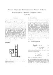
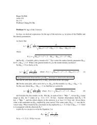
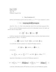
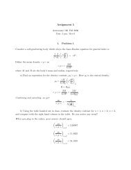
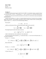
![Problem #1 [Structure Formation I: Radiation Era]](https://img.yumpu.com/37147371/1/190x245/problem-1-structure-formation-i-radiation-era.jpg?quality=85)