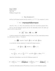
The Size, Structure, and Variability of Late-Type Stars Measured ...

5
leave the position of one telescope fixed, and move the other around to sample as much
of the Fourier space as possible. Actually, the rotation of the earth changes the effective
baseline throughout the course of the night and visibility can be recorded along a string of
baselines without moving either telescope. If the source happens to be circularly symmetric,
as might be expected for spherical objects such as stars, the visibility will also be circularly
symmetric with respect to [x,y], and the complex visibility defined in Equation 1.3 will
be real-valued. Thus, the visibility can be considered solely a function of the magnitude
of the baseline, or of the quantity known as spatial frequency which is the magnitude of
the baseline divided by the wavelength and expressed in terms of inverse radians. In this
case, the circularly symmetric intensity profile of the source could be reconstructed from
the fringe visibilities measured on baselines in a single direction.
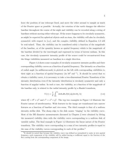
Figure 1.2 shows some examples of circularly symmetric intensity profiles and their
corresponding visibility curves as a function of spatial frequency. The intensity as a function
of radial angle (in milliarcseconds) is plotted on the left with corresponding visibilities to
their right as a function of spatial frequency (in 10 5 rad −1 ). It should be noted that to
obtain a visibility curve, it is necessary to take a two-dimensional Fourier Transform of the
intensity distribution even if the intensity distribution is circularly symmetric and only a
function of angular radius. In such a case, the visibility, as a function of the magnitude of
the baseline only, is related to the radial intensity profile by a Hankel transform,
V (r) = 1 F
∫ ∞
0
2πθ r dθ r I(θ r )J 0 (2πrθ r /λ) (1.4)
where θ 2 r = θ 2 + φ 2 and r 2 = x 2 + y 2 . The top two examples in Figure 1.2 illustrate the
Fourier nature of interferometry. Wide features in the image are transformed into narrow
features as a function of baseline and vice-versa. The third example is that of a uniform
intensity stellar disk. The sharp edge to the disk causes “ringing” in the visibility curve.
Most of the ISI diameter measurements discussed in Chapter 2 were obtained by fitting
the measured visibility data with the visibility curve corresponding to a uniform disk of
variable radius. The final example in Figure 1.2 illustrates the linear nature of the Fourier
transform. The visibility curve corresponding to a sum of two intensity profiles is equal to
the sum of the visibility curves corresponding to each of the profiles. 5
5 It should be noted that because the visibility curve was defined as normalized to unity at zero spatial
frequency, each component of the visibility will be added having a coefficient equal to the fraction of the
flux coming from the corresponding component of the image.