- Page 2 and 3:
Machine Learning Tom M. Mitchell Pr
- Page 4 and 5:
xvi PREFACE A third principle that
- Page 13 and 14:
CHAPTER INTRODUCTION Ever since com
- Page 15 and 16:
CHAPTER 1 INTRODUCITON 3 0 Learning
- Page 17 and 18:
CHAFTlB 1 INTRODUCTION 5 that allow
- Page 19 and 20:
1.2.2 Choosing the Target Function
- Page 21 and 22:
CHAPTER I INTRODUCTION 9 x5: the nu
- Page 23 and 24:
Thus, we seek the weights, or equiv
- Page 25 and 26:
could involve creating board positi
- Page 27 and 28:
the available training examples. Th
- Page 29 and 30:
0 Chapter 10 covers algorithms for
- Page 31 and 32:
ination of board features of your c
- Page 33 and 34:
CHAFER 2 CONCEm LEARNING AND THE GE
- Page 35 and 36:
When learning the target concept, t
- Page 37 and 38:
CHAPTER 2 CONCEPT LEARNING AND THE
- Page 39 and 40:
is needed. In the general case, as
- Page 41 and 42:
2.5 VERSION SPACES AND THE CANDIDAT
- Page 43 and 44:
{ 1 FIGURE 2.3 A version space w
- Page 45 and 46:
CHAPTER 2 CONCEET LEARNJNG AND THE
- Page 47 and 48:
C H m R 2 CONCEPT LEARNING AND THE
- Page 49 and 50:
CH.4PTF.R 2 CONCEFT LEARNING AND TH
- Page 51 and 52:
CHAPTER 2 CONCEPT LEARNING AND THE
- Page 53 and 54:
the power set of X? In general, the
- Page 55 and 56:
CHAFI%R 2 CONCEPT LEARNING AND THE
- Page 57 and 58:
CHAPTER 2 CONCEPT. LEARNING AND THE
- Page 59 and 60:
CHAFTER 2 CONCEPT LEARNING AND THE
- Page 61 and 62:
CHAPTER 2 CONCEPT LEARNING AND THE
- Page 63 and 64:
Hirsh, H. (1991). Theoretical under
- Page 65 and 66:
CHAPTER 3 DECISION TREE LEARNING 53
- Page 67 and 68:
CHAPTER 3 DECISION TREE LEARMNG 55
- Page 69 and 70:
CHAPTER 3 DECISION TREE LEARNING 57
- Page 71 and 72:
High wx CHAPTER 3 DECISION TREE LEA
- Page 73 and 74:
{Dl, D2, ..., Dl41 P+S-I Which attr
- Page 75 and 76:
3.6 INDUCTIVE BIAS IN DECISION TREE
- Page 77 and 78:
3.6.2 Why Prefer Short Hypotheses?
- Page 79 and 80:
easonable strategy, in fact it can
- Page 81 and 82:
Although the first of these approac
- Page 83 and 84:
multiple ways, then averaging the r
- Page 85 and 86:
CHAPTER 3 DECISION TREE LEARNING 73
- Page 87 and 88:
CHAPTER 3 DECISION TREE LEARNING 75
- Page 89 and 90:
CHAFER 3 DECISION TREE LEARNING 77
- Page 91 and 92:
C m 3 DECISION TREE LEARNING 79 Fay
- Page 93 and 94:
CHAPTER ARTIFICIAL NEURAL NETWORKS
- Page 95 and 96:
at normal speeds on public highways
- Page 97 and 98:
~t is also applicable to problems f
- Page 99 and 100:
FIGURE 43 A perceptron. A single pe
- Page 101 and 102:
this example. Notice the training r
- Page 103 and 104:
Gradient descent search determines
- Page 105 and 106:
- - CHAF'l'ER 4 ARTIFICIAL NEURAL N
- Page 107 and 108:
C H m R 4 ARTIFICIAL NEURAL NETWORK
- Page 109 and 110: CHAPTER 4 ARTIFICIAL NEURAL NETWORK
- Page 111 and 112: CHAPTER 4 ARTIFICIAL NEURAL NETWORK
- Page 113 and 114: CHAPTER 4 ARTIFICIAL NEURAL NETWORK
- Page 115 and 116: and combining this with Equations (
- Page 117 and 118: CHAPTER 4 ARTIFICIAL NEURAL NETWORK
- Page 119 and 120: Inputs Outputs Input 10000000 0 100
- Page 121 and 122: FIGURE 4.8 Learning the 8 x 3 x 8 N
- Page 123 and 124: CHAPTER 4 ARTIFICIAL NEURAL NETWORK
- Page 125 and 126: 30 x 32 resolution input images lef
- Page 127 and 128: left, (0,1,0,O) to encode a face lo
- Page 129 and 130: close to zero, as the bright face w
- Page 131 and 132: 4.8.2 Alternative Error Minimizatio
- Page 133 and 134: CHAPTER 4 ARTIFICIAL NEURAL NETWORK
- Page 135 and 136: BACKPROPAGATION searches the space
- Page 137 and 138: 4.6. Explain informally why the del
- Page 139 and 140: Mitchell, T. M., & Thrun, S. B. (19
- Page 141 and 142: the impact of possible pruning step
- Page 143 and 144: Here the notation Pr denotes that t
- Page 145 and 146: a A random variable can be viewed a
- Page 147 and 148: 5.3.2 The Binomial Distribution A g
- Page 149 and 150: In case the random variable Y is go
- Page 151 and 152: which is wide enough to contain 95%
- Page 153 and 154: intervals for discrete-valued hypot
- Page 155 and 156: Then as n + co, the distribution go
- Page 157 and 158: we might observe this difference in
- Page 159: 1. Partition the available data Do
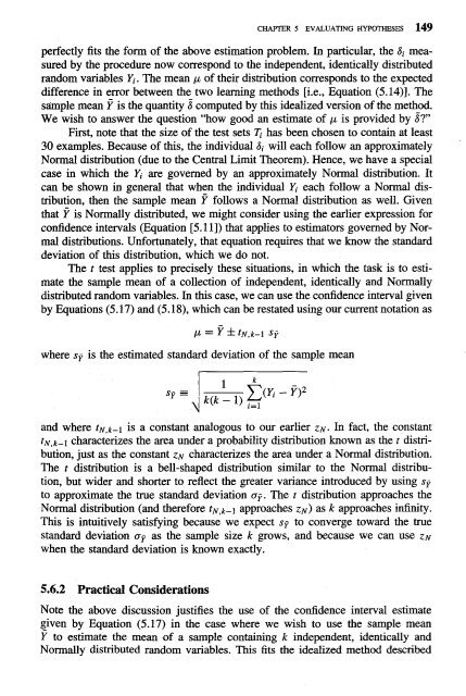
- Page 163 and 164: CHAFER 5 EVALUATING HYPOTHESES 151
- Page 165 and 166: Geman, S., Bienenstock, E., & Dours
- Page 167 and 168: CHAFER 6 BAYESIAN LEARNING 155 U Fo
- Page 169 and 170: CHAPTER 6 BAYESIAN LEARNING 157 As
- Page 171 and 172: . - Product rule: probability P(A A
- Page 173 and 174: CHAPTER 6 BAYESIAN LEARNING 161 Rec
- Page 175 and 176: CHAPTER 6 BAYESIAN LEARNING 163 of
- Page 177 and 178: CHAPTER 6 BAYESIAN LEARNING 165 a l
- Page 179 and 180: CHAPTER 6 BAYESIAN LEARNING 167 the
- Page 181 and 182: CHAPTER 6 BAYESIAN LEARNING 169 doe
- Page 183 and 184: CIUPlER 6 BAYESIAN LEARNING 171 sub
- Page 185 and 186: CHAPTER 6 BAYESIAN LEARNING 173 0 T
- Page 187 and 188: CHAFER 6 BAYESIAN LEARNING 175 the
- Page 189 and 190: 6.9 NAIVE BAYES CLASSIFIER CHAPTJZR
- Page 191 and 192: CHAETER 6 BAYESIAN LEARNING 179 Sim
- Page 193 and 194: -a- CHAPTER 6 BAYESIAN LEARNING 181
- Page 195 and 196: CHAPTER 6 BAYESIAN LEARNING 183 Exa
- Page 197 and 198: CHAPTER 6 BAYESIAN LEARNING 185 In
- Page 199 and 200: C H m R 6 BAYESIAN LEARNING 187 Fir
- Page 201 and 202: CHAPTER 6 BAYESIAN LEARNING 189 For
- Page 203 and 204: CHAPTER 6 BAYESIAN LEARNING 191 ord
- Page 205 and 206: CHAPTER 6 BAYESIAN LEARNING 193 max
- Page 207 and 208: CHAPTER 6 BAYESIAN LEARNING 195 Ste
- Page 209 and 210: 6.13 SUMMARY AND FURTHER READING Th
- Page 211 and 212:
CHAPTER 6 BAYESIAN LEARNING 199 pro
- Page 213 and 214:
CHAPTER COMPUTATIONAL LEARNING THEO
- Page 215 and 216:
CHAPTER 7 COMPUTATIONAL LEARNING TH
- Page 217 and 218:
C Instance space X Where c and h di
- Page 219 and 220:
usually more concerned with the num
- Page 221 and 222:
are drawn. Haussler (1988) provides
- Page 223 and 224:
CHAPTER 7 COMPUTATIONAL LEARNING TH
- Page 225 and 226:
C that contains every teachable con
- Page 227 and 228:
Instance space X FIGURE 73 A set of
- Page 229 and 230:
can show that it is at least 3, as
- Page 231 and 232:
The following theorem bounds the VC
- Page 233 and 234:
FIND-S: C CHAPTER 7 COMPUTATIONAL L
- Page 235 and 236:
We define the optimal mistake bound
- Page 237 and 238:
log' Rearranging terms yields which
- Page 239 and 240:
Current research on computational l
- Page 241 and 242:
(b) You now draw a new set of 100 i
- Page 243 and 244:
CHAPTER 8 INSTANCE-BASED LEARNING 2
- Page 245 and 246:
CHAPTER 8 INSTANCE-BASED LEARNING 2
- Page 247 and 248:
(i.e., on all axes in the Euclidean
- Page 249 and 250:
8.3.1 Locally Weighted Linear Regre
- Page 251 and 252:
C H m R 8 INSTANCE-BASED LEARNING 2
- Page 253 and 254:
CHAPTER 8 INSTANCEBASED LEARNING 24
- Page 255 and 256:
CHAPTER 8 INSTANCE-BASED LEARMNG 24
- Page 257 and 258:
CHAPTER 8 INSTANCE-BASED LEARNING 2
- Page 259 and 260:
A thorough discussion of radial bas
- Page 261 and 262:
CHAPTER GENETIC ALGORITHMS Genetic
- Page 263 and 264:
Fitness: A function that assigns an
- Page 265 and 266:
can then be represented by the foll
- Page 267 and 268:
the crossover point n is chosen at
- Page 269 and 270:
value of the target attribute c. Th
- Page 271 and 272:
In the above experiment, the two ne
- Page 273 and 274:
The second step above follows from
- Page 275 and 276:
FIGURE 9.2 Crossover operation appl
- Page 277 and 278:
0 (DU x y) (do until), which execut
- Page 279 and 280:
9.6.2 Baldwin Effect Although Lamar
- Page 281 and 282:
iteration, the most fit members of
- Page 283 and 284:
Belew, R. K., & Mitchell, M. (Eds.)
- Page 285 and 286:
Tumey, P. D., Whitley, D., & Anders
- Page 287 and 288:
As an example of first-order rule s
- Page 289 and 290:
10.2.1 General to Specific Beam Sea
- Page 291 and 292:
A few remarks on the LEARN-ONE-RULE
- Page 293 and 294:
decisions regarding preconditions o
- Page 295 and 296:
10.4 LEARNING FIRST-ORDER RULES In
- Page 297 and 298:
Every well-formed expression is com
- Page 299 and 300:
eralize the current disjunctive hyp
- Page 301 and 302:
Here let us also make the closed wo
- Page 303 and 304:
In the case of noise-free training
- Page 305 and 306:
(e.g., neural network) fits the dat
- Page 307 and 308:
C : KnowMaterial v -Study C: KnowMa
- Page 309 and 310:
CHAPTER 10 LEARNING SETS OF RULES 2
- Page 311 and 312:
In contrast, the generate-and-test
- Page 313 and 314:
which enable the user to specify th
- Page 315 and 316:
Wrobel (1992) use rule schemata in
- Page 317 and 318:
De Raedt, L., & Bruynooghe, M. (199
- Page 319 and 320:
CHAPTER ANALYTICAL LEARNING Inducti
- Page 321 and 322:
What is interesting about this ches
- Page 323 and 324:
Given: rn Instance space X: Each in
- Page 325 and 326:
theories to automatically improve p
- Page 327 and 328:
Explanation: Training Example: FIGU
- Page 329 and 330:
FIGURE 11.3 Computing the weakest p
- Page 331 and 332:
example that is not yet covered by
- Page 333 and 334:
contain no description of such a pr
- Page 335 and 336:
additional detail that must be cons
- Page 337 and 338:
CHAPTER 11 ANALYTICAL LEARNING 325
- Page 339 and 340:
explaining to itself the reason for
- Page 341 and 342:
that fits the learner's prior knowl
- Page 343 and 344:
Height (Joe, Short) Height(Sue, Sho
- Page 345 and 346:
CHAF'TER 11 ANALYTICAL LEARNING 333
- Page 347 and 348:
CHAPTER 12 COMBINING INDUCTIVE AND
- Page 349 and 350:
CHAF'TER 12 COMBINING INDUCTIVE AND
- Page 351 and 352:
12.2.2 Hypothesis Space Search CAAP
- Page 353 and 354:
- KBANN(Domain-Theory, Training_Exa
- Page 355 and 356:
CHAPTER 12 COMBINING INDUCTIVE AND
- Page 357 and 358:
CHAPTER 12 COMBINING INDUCTIVE AND
- Page 359 and 360:
CHAF'TER 12 COMBINING INDUCTIVE AND
- Page 361 and 362:
CHAPTER 12 COMBINING INDUCTIVE AND
- Page 363 and 364:
Hypothesis Space Hypotheses that ma
- Page 365 and 366:
CHAFER 12 COMBINING INDUCTIVE AND A
- Page 367 and 368:
CHAPTER 12 COMBmG INDUCTIVE AND ANA
- Page 369 and 370:
CHAPTER 12 COMBINING INDUCTIVE AND
- Page 371 and 372:
CHAPTER 12 COMBINING INDUCTIVE AND
- Page 373 and 374:
Hypothesis Space 1 Hypotheses thatf
- Page 375 and 376:
y first order Horn clauses to learn
- Page 377 and 378:
Craven, M. W., & Shavlik, J. W. (19
- Page 379 and 380:
CHAPTER REINFORCEMENT LEARNING Rein
- Page 381 and 382:
has or does not have prior knowledg
- Page 383 and 384:
CHAPTER 13 REINFORCEMENT LEARNING 3
- Page 385 and 386:
CHAPTER 13 REINFORCEMENT LEARNING 3
- Page 387 and 388:
CHAPTER 13 REINFORCEMENT LEARNJNG 3
- Page 389 and 390:
CHAPTER 13 REINFORCEMENT LEARNING 3
- Page 391 and 392:
CHAPTER 13 REINFORCEMENT LEARNING 3
- Page 393 and 394:
CHAPTER 13 REINFORCEMENT LEARNING 3
- Page 395 and 396:
While Q learning and related reinfo
- Page 397 and 398:
a neural network reinforcement lear
- Page 399 and 400:
CHAFER 13 REINFORCEMENT LEARNING 38
- Page 401 and 402:
CHaPrER 13 REINFORCEMENT LEARNING 3
- Page 403 and 404:
APPENDIX NOTATION Below is a summar
- Page 405 and 406:
INDEXES
- Page 407 and 408:
in KBANN algorithm, 343-344 optimiz
- Page 409 and 410:
leave-one-out, 235 in neural networ
- Page 411 and 412:
extensions to, 258-259 ID5R algorit
- Page 413 and 414:
of LMS algorithm, 64 of ROTE-LEARNE
- Page 415 and 416:
prediction of probabilities with, 1
- Page 417 and 418:
Probability distribution, 133. See
- Page 419 and 420:
Split infomation, 73-74 Squashing f