Determination of the material characteristics by means of a high ...

Determination of the Material Characteristics by Means of a
High Speed Tensile Test – Experiments and Simulations
O. K. Demir 1 , O. Höhling 1 , D. Risch 1 , A. Brosius 1 , A. E. Tekkaya 1
1 Institute of Forming Technology and Lightweight Construction (IUL) – Technische Universität Dortmund,
Baroper Str. 301, 44227 Dortmund
URL: www.iul.eu
e-mail: koray.demir@iul.uni-dortmund.de;
ortrun.hoehling@iul.uni-dortmund.de;
desiree.risch@iul.uni-dortmund.de;
alexander.brosius@iul.uni-dortmund.de;
erman.tekkaya@iul.uni-dortmund.de
ABSTRACT: Three high speed tensile tests of the aluminum alloy AlMg3 and finite element (FE) simulations
of these tests were performed. The strain rate dependency parameters for the Cowper-Symonds material
model, which minimize the difference between measured and simulated displacement results, were determined.
The verification of the determined parameters by means of strain distribution comparisons between an
additional experiment and its simulation revealed the necessity for further consideration of the parameters.
Keywords: High speed tensile test, material characterisation, finite element simulation
1 INTRODUCTION & MOTIVATION
The enhanced formability of aluminum at high strain
rates makes high speed forming processes of this
material more and more attractive, which, in turn,
increases the necessity for a better understanding of
these processes. FE simulations are widely used for
this aim; however, due to strain rate sensitivity of
aluminum and its alloys at high strain rates knowledge
of material data that is valid at high strain rates
is essential in order to obtain accurate results in
simulations.
One way to acquire this information is high speed
sheet tensile testing, which is known as one of the
most difficult ways of material evaluation [1] due to
mechanical vibrations complicating force measurements,
high inertial forces, adiabatic increase of
temperature, and continuous variation of local and
temporary strain and strain rate during the test [2].
In this study, an inverse engineering method was
used in order to avoid these difficulties of the test
with the help of FE simulations. By means of an
optimization loop the material parameters of AlMg3
for the viscoplastic material model of Cowper and
Symonds [3] were determined.
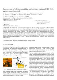
2 DESCRIPTION OF THE EXPERIMENTAL &
NUMERICAL SETUP
2.1 Experimental Setup & Measurement Systems
The experimental setup for the analysed high speed
tensile tests is presented in figure 1. The specimen is
fixed with pins between the upper and lower plunger
and this plunger-specimen-unit is positioned at the
upper end of the acceleration pipe. The test is started
by dropping the plunger-specimen-unit. In order to
achieve velocities up to 25 m/s, which are higher
than those realized merely by gravity (approx. 10
m/s), an additional pressure supply can be used. At
the lower end of the acceleration tube the upper
plunger is suddenly stopped by an anvil, while the
specimen is elongated due to the continuation of the
lower plunger’s movement caused by inertia.
In order to determine the course of this movement,
an online measurement system using the effect of
shadowing a light beam is applied (see figure 2).
The principle is well known from several publications
in the field of high speed forming of tubes.
With modern electronic components a measurement
system has been designed and adapted to the current
setup [5].

adapted measurement devices will be the input as
well as reference for the numerical analysis.
2.2 Numerical Setup
Fig. 1 Experimental setup and measurement systems
The system consists of a laser beam which is expanded
to a line, parallelized by a lens, and received
by a so called Position Sensitive Device (PSD). During
the deformation process the lower plunger
moves between laser and receiver, partly shadowing
the laser light so that the quantity of light changes
directly proportional to the displacement of the
lower plunger.
Fig. 2 Principle of Laser-PSD
An additional measurement facility (see figure 1),
which is adapted to the testing device, is the high
speed camera HSFC.pro (company PCO, Germany).
This camera is able to take eight pictures within a
variable time interval reaching from a tenth of a microsecond
to seconds. Figure 6 shows a series of
four pictures from the whole sequence. Furthermore,
a stochastic pattern can be recognized which is necessary
in order to do a strain analysis with the
Aramis system developed by the GOM company [6].
The last adapted measurement device is a light barrier
which is integrated in the acceleration pipe in
order to trigger the high speed camera. Additionally,
using again the effect of shadowing a light beam, it
is possible to determine the fall velocity of the
plunger-specimen-unit. The experimental data of all
The FE simulations were performed using the dynamic
explicit three dimensional solver of the commercial
code LS-DYNA, employing brick-shaped
elements with eight nodes, single integration point,
and hourglass control.
The necessity for the dynamic calculation arises
from the fact that the transit times for the stress
waves travelling along the specimen are long with
respect to the duration of the application of tensile
forces. During the experiments the fracture of the
specimen occurs in certain cases after approx.
300 μs, while a mechanical wave travels back and
forth along the specimen in 24 μs, which means that
a stress wave moves back and forth only 12 times
during the whole test. This prevents the equilibrium
of forces in the specimen from evolving and makes a
static assumption useless.
The assumption of linear elastic material behaviour
was made for the pins, while the viscoplastic constitutive
model developed by Cowper and Symonds
was used for the plastic deformation of the specimen,
neglecting the effect of adiabatic heating. This
model is selected based on the low number of variables,
which means a reduced number of simulations
during the optimization loops. The application of the
Cowper-Symonds model in LS-DYNA requires the
elastic constants and the quasi-static (q-s) flow curve
of the material and scales the given flow stress values
with a factor calculated by eq. (1) given below:
⎛ ε ⎞
Scale factor = 1+ ⎜ ⎟
⎝C
⎠
1
p
, (1)
where ε is the strain rate and C and p are the
Cowper-Symonds strain rate parameters. The q-s
flow curve of AlMg3 for the simulations was obtained
by a conventional tension test.
A representative mesh of the specimen and the dimensions
of the model can be seen in figure 3.
46,000 elements have been used for the numerical
model of the specimen. The front pin is attached to a
point mass, which represents the lower plunger.
While the whole model (specimen, pins, and the
plunger) has a certain initial velocity in x-direction,
the nodes in the front region of the back pin are constrained
in x-direction, which represents the impact
between the back pin and the plunger that occurs

when the plunger stops suddenly.
In order to simulate a given experiment, the velocity
of the plunger-specimen unit just before the impact
needs to be measured. This velocity is transferred to
the FE simulation as an initial condition. The outputs
of the simulation and experiment can be compared
considering the displacement course of the lower
plunger.
3 RESULTS
3.1 Course of Plunger Displacement
Figure 4 reveals the experiment results and simulation
results when C=p=0 (q-s flow curve is used)
and when C=850 and p=0.03.
Fig. 3 FE model
2.3 Determination of the Material Parameters
In order to determine the C-p couple equating the
displacement results of a simulation to the corresponding
experiment, first, two simulations were
performed with two initial guesses of the C-p couple.
The following guesses were calculated by a simplex-based
optimization algorithm developed by
Nelder and Mead [4] until the objective function
given below is minimized:
2
f( C, p) = ∑ ( uexp
⋅uexp
−usim
⋅u sim)
, (2)
where u and u represent the displacement and velocity
of the lower plunger and subscripts “exp” and
“sim” stand for experiment and simulation, respectively.
The objective function was evaluated by taking
only experimental data until fracture into account.
There can be more than one C-p couple that makes a
simulation result coincident with the corresponding
measurement. Furthermore, the C-p couple determined
for an experiment depends on the initial
guesses supplied by the user and it is not necessarily
valid for other experiments performed at different
velocities. Here, our aim was to determine a C-p
couple valid for all experiments at hand. The reliability
of the determined couple is directly proportional
to the number of experiment-simulation pairs
taken into account during the optimization process.
For this study, three experiments were performed at:
11.4 m/s, 15.9 m/s, and 22.6 m/s.
Fig. 4 Measured and calculated plunger displacement courses
When the tests were simulated using the q-s flow
curve of the material, the simulations overestimated
the measured displacements of the lower plunger
severely, as expected. The utilization of the mentioned
C-p couple reduced the maximum error values
until fracture to 5.9%, 1.9%, and 4.3% for the
cases of 11.4 m/s, 15.9 m/s, and 22.6 m/s initial velocities,
respectively.
As can be seen in figure 5, with these parameters the
material gains a very strong strain rate dependency.
The parameter p decides the sensitivity of the scale
factor to strain rate. A very small value, as the one
found, leads to an extreme sensitivity and very large
scale factors above a strain rate of 880 s -1 . The importance
of the factor C arises at this point: it determines
this critical strain rate value, above which the
calculated scale factors are very large. Hence, for
small values of p the scale factor is also very sensitive
to C, which is another disadvantage of the determined
parameter couple.
Fig. 5 Scale factor with respect to strain rate and p

3.2 Course of Strain Distribution
In order to validate the determined material parameters,
an additional experiment with a velocity of
9.2 m/s, which is outside the range of the other three
velocities, was carried out and eight pictures were
taken using the high speed camera. Four representative
photos are given in figure 6.
The elongation at fracture measured after the experiment
was 4 mm. Since the high speed camera
and the displacement measurement setup cannot be
used simultaneously the according time period must
be approximated. According to an extrapolation of
previous experiment results, a duration of 600 μs
was estimated. Thus, the time at figure 6c was assumed
to be 600 µs due to the occurring fracture.
Knowing the time period between two photos being
100 μs, the time for all the photos can be deduced.
Fig. 6 Photos from a high speed tensile test. a) initial state, b)
elongation, c) fracture, and d) the state after the fracture
Next, the strain distribution on the surface of the
specimen along the centreline was analysed using
the Aramis system and the results were compared to
the simulations. Figure 7 shows the comparison.
t=500 μs in the necking region. These changes make
the simulation results resemble the experimental
results qualitatively, but the strain evolution, obvious
in the experiment data, cannot be acquired in the
simulation.
This can be explained by errors in measuring the
initial specimen velocity, measuring strains, or approximating
the moments, when the photos were
taken. It might also indicate that the Cowper-
Symonds model or the determined parameters are
unsuitable for modelling the behaviour of AlMg3.
4 SUMMARY
A combined experimental and numerical approach
for determining the material behaviour of AlMg3 at
high strain rates was tested. Therefore, a high speed
tensile test including several measurement systems
was realized. FE simulations were carried out in
order to find the Cowper-Symonds material constants
by means of an inverse analysis. The determined
constants are pretty successful in predicting
experimental displacements, but the strain results
need more consideration. Applying the same methodology
with more experiments, or verifying the
used material model or measurement techniques are
conceivable alternatives for further research.
ACKNOWLEDGEMENTS
The authors would like to thank the German Research Foundation
(DFG) for its financial support of the work reported here,
acquired within the scope of Research Unit FOR 443.
Fig. 7 Strain distribution courses. a) experiment results, b)
trendlines of experiment results, c) simulation results (C=p=0),
d) simulation results (C=880, p=0.03)
Applying the parameters prevents strain localization
that takes place at t=300 μs around x=1, and later at
REFERENCES
1. P. Larour, A. Rusinek, J.R. Klepaczko and W. Bleck,
‘Effects of Strain Rate and Identification of Material
Constants for Three Automative Steels’, Steel Research
Int., 78, (2007) 348-358
2. M. Kleiner and A. Brosius, ‘Determination of Flow
Curves at High Strain Rates using the Electromagnetic
Forming Process and an Iterative Finite Element Simulation
Scheme’, CIRP Annals - Manufacturing Technology,
55, (2006) 267-270
3. P.S. Symonds, ‘Survey of Methods of Analysis for plastic
deformation of structures under dynamic loading’,
Technical Report, Brown University, 1967
4. J.A. Nelder, R. Mead, ‘A Simplex Method for Function
Minimization’, Computer Journal, 7, (1965) 308-313
5. M. Badelt, C. Beerwald, A. Brosius and M. Kleiner,
Process Analysis of Electromagnetic Sheet Metal Forming
by Online-Measurement and Finite Element Simulation.
Proc. of the 6th ESAFORM, 2003, 123-126
6. www.gom.com