Stability Analysis of an All-Electric Ship MVDC Power Distribution ...

More documents

Recommendations

Info

î in ˆ =0 i load 100 Bode plot of Z Z bus_FB Z S Z S vˆg vg _ FB g Z in _ FB G ii _ FB iˆ G load vˆ Z out _ FB vˆo Magnitude (dB) 50 0 -50 -100 90 Wres Range of frequencies where Passivity is violated Z in_FB (a) ˆ =0 i load Phase (deg) 0 -90 -180 Z S vˆg î in Z in _ FB Z damp G ii _ FB G G iˆ vd_ PICM id_ PICM load G vˆ Z vg_ g damp FB vˆ g Z out _ FB vˆo -270 -360 10 -1 10 0 10 1 10 2 10 3 10 4 10 5 10 6 250 Frequency (Hz) (a) Nyquist plot of Z Z bus _ FB 200 Z S Passivity Condition Violated 150 (b) 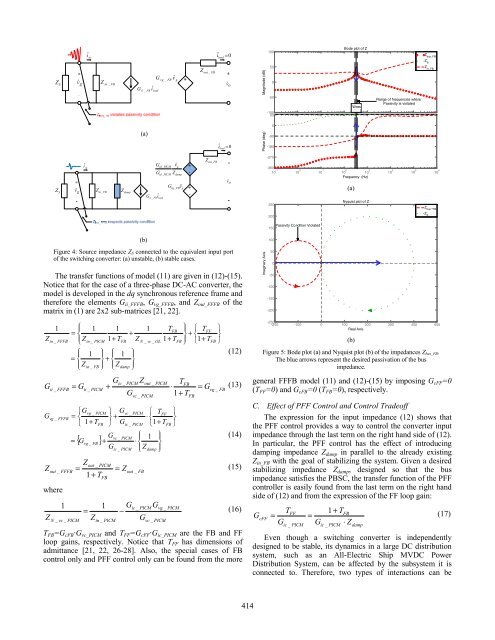Figure 4: Source impedance Z S connected to the equivalent input port of the switching converter: (a) unstable, (b) stable cases. The transfer functions of model (11) are given in (12)-(15). Notice that for the case of a three-phase DC-AC converter, the model is developed in the dq synchronous reference frame and therefore the elements G ii_FFFB , G vg_FFFB , and Z out_FFFB of the matrix in (1) are 2x2 sub-matrices [21, 22]. Z G G Z 1 in _ FFFB ⎪⎧ 1 = ⎨ ⎪⎩ Zin _ ⎪⎧ 1 = ⎨ ⎪⎩ Zin _ PICM FB 1 1+ T FB ⎪⎫ ⎪⎧ 1 ⎬ + ⎨ ⎪⎭ ⎪⎩ Z G damp + Z ⎪⎫ ⎬ ⎪⎭ 1 N _ vc _ OL Z TFB 1+ T FB ⎪⎫ ⎧ TFF ⎬ + ⎨ ⎪⎭ ⎩1+ T FB ⎫ ⎬ ⎭ (12) ic _ PICM out _ PICM FB ii _ FFFB = Gii _ PICM + ⋅ = G (13) vg _ FB Gvc _ PICM 1+ TFB vg _ FFFB ⎧Gvg _ = ⎨ ⎩ 1+ T = { G } vg _ FB Z PICM FB ⎫ ⎬ + ⎭ G + G G G vc _ PICM ic _ PICM ⎧ TFF ⋅ ⎨ ⎩1+ T ⎪⎧ 1 ⎪⎫ ⋅ ⎨ ⎬ ⎪⎩ Zdamp ⎪⎭ vc _ PICM ic _ PICM FB ⎫ ⎬ ⎭ T (14) out _ PICM out _ FFFB = = Z (15) out _ FB 1+ TFB where Z 1 1 G ic _ PICM vg _ PICM = − (16) N _ vc _ PICM Zin _ PICM Gvc _ PICM T FB =G cFB·G vc_PICM and T FF =G cFF·G ic_PICM are the FB and FF loop gains, respectively. Notice that T FF has dimensions of admittance [21, 22, 26-28]. Also, the special cases of FB control only and PFF control only can be found from the more G Imaginary Axis 100 50 0 -50 -100 -150 -200 -250 -200 -100 0 100 200 300 400 500 Real Axis (b) Figure 5: Bode plot (a) and Nyquist plot (b) of the impedances Z bus_FB. The blue arrows represent the desired passivation of the bus impedance. general FFFB model (11) and (12)-(15) by imposing G cFF =0 (T FF =0) and G cFB =0 (T FB =0), respectively. C. Effect of PFF Control and Control Tradeoff The expression for the input impedance (12) shows that the PFF control provides a way to control the converter input impedance through the last term on the right hand side of (12). In particular, the PFF control has the effect of introducing damping impedance Z damp in parallel to the already existing Z in_FB with the goal of stabilizing the system. Given a desired stabilizing impedance Z damp , designed so that the bus impedance satisfies the PBSC, the transfer function of the PFF controller is easily found from the last term on the right hand side of (12) and from the expression of the FF loop gain: G cFF T = G FF ic _ PICM = G 1 + TFB (17) ic _ PICM ⋅ Z damp Even though a switching converter is independently designed to be stable, its dynamics in a large DC distribution system, such as an All-Electric Ship MVDC Power Distribution System, can be affected by the subsystem it is connected to. Therefore, two types of interactions can be 414
identified: the source subsystem interaction, and the load subsystem interaction. In this paper, the focus is on the source subsystem interaction problem, i.e., a degradation of the closed-loop stability of a switching converter when it is fed by a DC voltage source subsystem with finite Thévenin impedance Z S . Fig. 4a shows the two-port network terminal model [29, 30], directly drawn from model (11), for the case of FB only (G cFF (s)=0) with a non-ideal source impedance Z S . In terms of passivity concept, passivity condition for Z bus_FB is usually violated around ω res , i.e. the frequency where Z bus_FB exhibits resonance, as Fig. 5 shows. Impedance Z bus_FB follows the output impedance of the source subsystem Z S everywhere except around the range of frequencies where it exhibits resonance (in the parallel combination the smaller impedance dominates). To solve the passivity condition violation, i.e. to bring Z bus to the RHP so that it exhibits positive real part at frequencies around ω res , the PFF control is added to the conventional FB control according Fig. 3a. If Z damp is designed so that (18) is satisfied, the passivity violation can be solved. Z 1 bus _ FFFB 1 = Z S ⎧ 1 ⎪ ⎪ Z S ⎪ 1 ≈ ⎨ ⎪Z ⎪ 1 ⎪ ⎩ Z S 1 + Z damp in _ FB 1 + Z at low frequencies at high damp atω = ω res frequencies (18) Z bus_FFFB is the bus impedance resulting from the addition of the PFF control. In other words, (18) shows that if Z damp is designed so that it dominates at ω res (note, again, that in the parallel combination the smallest impedance dominates), it can provide the desired passivation effect (see blue arrows in Fig. 5a), i.e. -90°≤arg[Z bus_FFFB (jω res )]≤90° while leaving the bus impedance unchanged everywhere else. This is also equivalent to moving the Nyquist plot of the bus impedance from the LHP to the RHP, as the blue arrow in Fig. 5b indicates. Fig. 4 shows an equivalent model for the system under FB control only (a) and under FFFB control (b). The feed-forward action introduces two additional elements, impedance Z damp on the source side and a controlled voltage source on the output side. The impedance Z damp stabilizes the bus, but at a cost: the output side voltage source has a negative effect on audio susceptibility. This represents a tradeoff between stability improvement and output performance degradation. In fact, as Fig. 5 also depicts, on the one hand the addition of Z damp small in magnitude at ω res (so that it dominates to solve the passivity violation problem) is desired for stability improvement purposes, on the other hand it negatively affects the audiosusceptibility transfer function (14). For this reason, Z damp should be carefully chosen. Notice that Z damp can be chosen to be either passive or active impedance. What it important is that it should be chosen so that ||Z damp (jω res )|| be not too small, but small enough to dominate the bus impedance at ω res . A PGM‐M PGM‐M PGM‐M PGM‐M PCM‐A PDM‐B PCM‐B PCM‐B PCM‐B PMM PDM‐A In‐Zone Distribution PMM PCM‐B PCM‐B PCM‐B PCM‐A Figure 6: Traditional 3-PDM IPS Architecture, with the two zones that will be simulated. good rule of the thumb is to choose Z damp so that ||Z bus_FB (jω res )|| dB is 20-25 dB larger than ||Z damp (jω res )|| dB . Of course, condition (18) must be respected as well. In particular, it is desired that arg[Z bus_FFFB (jω res )] lies as close as possible to 0° so that the system has a good passivity margin (it is far away from the passivity boundary). IV. SIMULATION RESULTS In this section, the PBSC is validated by using a switching model of a MVDC bus system built in Simulink. The simulated system is a power down-scaled portion of one of the possible Integrated Power System (IPS) architectures that have been proposed in [31]. The architecture taken into consideration in this paper is the traditional three Propulsion Distribution Module (PDM) ISP architecture, shown in Fig 6. PDM-A is a HVDC bus (10 KV), PGMs are high frequency Power Generation Modules with rectifier units, PMMs are Propulsion Motor Modules, PDM-B is a MVDC bus (1000 V), and the Power Conversion Modules (PCMs) are switching converters. Two portions of the system in Fig. 6 will be simulated, represented by areas within the red and blue dashed lines. Fig. 7 shows the system switching model built in Simulink. The area within the red dashed line is a cascade of a PICM-FB-controlled buck converter and a PICM-FFFBcontrolled three-phase voltage source inverter (VSI). The controller of the VSI has a PFF controller in addition to the conventional FB controller as shown in Fig. 8. The area within the blue dashed line is the same system with the addition of a high bandwidth CPL, representative of another switching converter or a pulsed load, like a radar or rail-gun for future naval combatants. Specifications for both buck converter and VSI are also reported in Fig. 7. The PFF control was designed to actively introduce the following damping impedance at the VSI input port. 1 Zdamp = Rb + sLb + (19) sCb where R b =21.34Ω, L b =17.88mH, and C b =157.19µF. The PFF controller transfer function is then calculated from (17). PDM‐B 415
Page 1 and 2: Stability Analysis of an All-Electr
Page 3: Forward (PFF) control. The PFF cont
Page 7 and 8: 240 230 220 210 200 190 180 170 160
Page 9: [12] Xiaogang Feng; Zhihong Ye; Kun

Stability Analysis of an All-Electric Ship MVDC Power Distribution ...

You also want an ePaper? Increase the reach of your titles

Delete template?

Save as template?