Hydrostatic Consistency in Sigma Coordinate Ocean Models - NPS ...

Hydrostatic Consistency in Sigma
Coordinate Ocean Models
Peter C. Chu and Chenwu Fan
Naval Ocean Analysis and Prediction Laboratory, Department of Oceanography
Naval Postgraduate School, Monterey, California
1

Abstract
Truncation error and hydrostatic inconsistency at steep topography are two
concerns in sigma coordinate ocean models due to the horizontal pressure gradient being
difference of two large terms. A consensus is reached in the ocean modeling community
on the first concern (truncation error), but not on the second concern (hydrostatic
inconsistency). Since the integration of the pressure gradient over a finite volume equals
the integration of the pressure over the surface of that volume (always dynamically
consistent), dynamical analysis on finite volumes is used to determine the hydrostatic
consistency of a sigma coordinate ocean model. A discrete, hydrostatically consistent
scheme is obtained for the sigma coordinate ocean models. Comparison between finitevolume
and finite-difference approaches leads to the conclusion that a Boussinesq,
hydrostatic, sigma coordinate ocean model with second-order staggered scheme is always
hydrostatically consistent. Guidance for improving numerical accuracy is also provided.
2

1. Introduction
In regional oceanic (or atmospheric) prediction models the effects of bottom
topography must be taken into account and a continuous topography is implied in terrainfollowing
sigma coordinates. The water column is divided into the same number of grid
cells independence of depth. We restrict attention to two dimensions. Let (x, z) denote
Cartesian coordinates and (x*,
σ ) be the sigma coordinates. The conventional
relationship between z- and sigma-coordinates is given by
x = x*, z = σ H( x*)
, (1)
where z and σ increase vertically upward such that z = σ = 0 at the surface and σ =−1,
z = -H at the bottom. The horizontal pressure gradient can be computed by
∂p ∂p*
σ ∂H
∂p *
= −
. (2)
∂x ∂x* H ∂x*
∂σ
The horizontal pressure gradient becomes difference between two large terms, which may
cause two problems: (1) truncation error at steep topography [e.g., Gary, 1973; Haney,
1991; Mellor et al., 1994, 1998; McCalpin, 1994; Chu and Fan, 1997, 1998; Song, 1998],
and (2) hydrostatic inconsistency [e.g., Mesinger, 1984; Haney, 1991].
A consensus is reached in the ocean modeling community that the first problem
does exist and several methods have been suggested to reduce the truncation errors to
acceptable levels: (1) smoothing topography [e.g., Chu and Fan, 2001], (2) subtracting a
mean vertical density profile before calculating the gradient [Gary, 1973], (3) bringing
certain symmetries of the continuous forms into the discrete level to ensure cancellations
of these terms such as the density Jacobian scheme [e.g., Mellor et al. 1998; Song, 1998;
3

Song and Wright, 1998], (4) increasing numerical accuracy [e.g., McCalpin, 1994; Chu
and Fan, 1997, 1998, 1999, 2000, 2001], (5) changing the grid from a sigma grid to a z-
level grid before calculating the horizontal pressure gradient [e.g., Stelling and van
Kester, 1994]. Kliem and Pietrzak [1999] claimed that the z-level based pressure gradient
calculation is the most simple and effective means to reduce the pressure gradient errors.
However, Ezer et al. [2002] found that the density Jacobian scheme is more preferable.
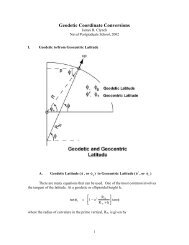
No consensus is reached on whether the second problem exists. Based on the
earlier work for atmospheric models [e.g., Messiger, 1982], Haney [1991] pointed out
that the vertical discretization in sigma coordinate ocean models ( δσ ) should satisfy the
hydrostatic consistency condition,
σδ H x
r ≡ < 1
(3)
H δσ
to keep the computational stability. Here r is the hydrostatic consistency parameter;
δ H x
is the horizontal change in depth of adjacent grid cells; and
δσ is the vertical cell
size associated with a sigma grid, δxδσ . However, Mellor et al. [1994] thought that r is
just another measure of the numerical accuracy after conducting a numerical simulation
for the North Atlantic Ocean using the Princeton Ocean Model with r = 3. More
numerical experiments with various schemes for the seamount test case [e.g., Ezer et al.,
2002] were conducted to show convergent solutions with r = 14.2. These experiments
show that the condition (3) is not the ultimate condition for numerical calculation, but the
indication of the first (second) term in the righthand-side of (2) is larger if r < 1 (r > 1).
Does the hydrostatic inconsistency regarding to the computational instability
really exist? We use the finite volume integration approach [Lin, 1997] to reexamine the
concept of hydrostatic consistency (regarding the stability) in this paper. A fully,
4

hydrostatically consistent (i.e., hydrostatically stable) grid scheme is developed for sigma
coordinate ocean models. This scheme provides a criterion for the identification of
hydrostatic consistency for various finite difference schemes. The outline of this part is as
follows: Description of the hydrostatic consistency is given in section 2. A
hydrostatically consistent staggered scheme for horizontal pressure gradient is given in
Section 3. Evidence of second-order staggered sigma ocean model is always
hydrostatically consistent is given in Sections 4 and 5. In section 6, the conclusions are
presented.
2. Hydrostatic Consistency
Let the flow field change in x– z plane only (Fig. 1). A finite volume (trapezoidal
cylinder) is considered with the length of L y (in the y-direction) and the cross-section
represented by the shaded region (trapezoid) in Figure 1. The resultant pressure force (F)
acting on the finite volume is computed as follows:
∫
F= L p n ds
(4)
y
C
where p is the pressure, C represents the four boundaries, n denotes the normal unit
vector pointing inward, and ds is an element of the boundary. The contour integral is
taken counter-clockwise along the peripheral of the volume element. The pressure force
exerts on boundaries of the finite-volume with p w , p e , p u , and p l on the west, east, upper,
and lower sides. The horizontal (F x ) and vertical (F z ) components of the resultant
pressure force are computed by
2 3 4 1
Fx L ⎛
⎞
=−
y⎜∫ pdz
l
+ ∫ pedz+ ∫ pudz+
∫ pwdz⎟, (5)
⎝ 1 2 3 4 ⎠
5

2 4
Fz L ⎛
⎞
=
y⎜∫ pdx
l
+ ∫ pudx⎟, (6)
⎝ 1 3 ⎠
where points 1, 2, 3, and 4 are the four vertices of the finite volume. For hydrostatic
balanced models, the following condition must hold
Fz
= g∆m
, (7)
where g is the gravitational acceleration,
∆m
is the mass of the finite volume. Equation
(7) states that the vertical component of the resultant pressure force acting on the finite
volume exactly balances the total weight of the finite volume.
For a Boussinesq, hydrostatic ocean model, the pressure field is given by
0
p = p + ρ0 gη+ g∫ ρ( x, z', t)
dz ', (8)
atm
z
where
patm
is the atmospheric pressure at the ocean surface, ρ 0
is the characteristic
density, and η is the surface elevation. Substitution of (8) into (6) leads to
2 0 4 0
⎛
⎞
Fz
= gLy⎜∫∫ρ( x, z ', t) dz ' dx + ∫∫ρ( x, z ', t) dz ' dx ⎟
⎝ 1 z
3 z
⎠
∫∫
= gL ρ( x, z ', t) dz ' dx = g∆m,
y
∆S
(9)
where
∆S is the area of the trapezoid (Fig. 1) computed by
∆ S = ( xi+ 1
−xi) ⋅ ( zi, k
+ zi+ 1, k
−zi, k+
1
− zi+
1, k+ 1)
, zik ,
= Hi⋅σ
k. (10)
Eq.(9) indicates that the finite-volume discretization guarantees the hydrostatic balance in
Boussinesq, hydrostatic ocean models. Using (5) the horizontal pressure gradient is
computed by
6

2 3 4 1
∂p
F 1 ⎛
⎞
≡
x = − ⎜ pldz + pedz + pudz + pwdz
⎟
∂x Ly∆S ∆S
⎝ 1 2 3 4 ⎠
∫ ∫ ∫ ∫ . (11)
If the horizontal pressure gradient is represented by (11), the model is conserved and
hydrostatic inconsistency does not exist. Thus, deviation from the hydrostatic consistency
becomes deviation of the horizontal pressure gradient computation from (11).
3. Staggered Grid
The staggered grid is represented in Figure 1 with the velocity at the center of the
volume and pressure at the four vertices. Discretization of the horizontal pressure
gradient with the finite-volume consideration (11) is given by
∆ p 1 = ⎡ pl( zi+ 1, k+ 1 − zi, k+ 1) + pe( zi+ 1, k − zi+ 1, k+ 1
) + pu( zi, k − zi+ 1, k) + pw(
zi, k+
1
zi,
k ⎤
x S
⎣
− )
∆ ∆
⎦, (12)
where pl, pe, pu,
p
w
are the mean values of pressure at the four sides of the trapezoid.
Equation (12) is the criterion for justifying the hydrostatic consistency for ocean model
with staggered grid. If the horizontal pressure gradient in sigma coordinates (2) can be
represented by (12), the model is hydrostatically consistent. Otherwise the model may be
hydrostatically inconsistent. For ocean models with C-grid, the two consecutive finitevolumes
are considered as one volume (Fig. 2). The hydrostatic consistency can be easily
evaluated on these finite-volumes.
4. Second-Order Accuracy
For the second-order staggered grid, pl, pe, pu,
p
w, are taken as the arithmetic
means of pressure at the two vertices,
p
w
=
p
+ p
ik , ik , + 1 ,
2
p
e
=
p
+ p
i+ 1, k i+
1, k + 1
,
2
7

p
l
=
p
+ p
ik , + 1 i+
1, k+ 1
ik , i+
1, k
u
2
p
=
p
+ p
2
. (13)
Substitution of (13) into (12) leads to
( pi+ 1, k+ 1
− pi, k) ⋅( Hi+ 1σk − Hiσk+ 1) + ( pi+ 1, k
− pi, k+ 1) ⋅( Hiσk −Hi+ 1σk+
1)
⎛∆p
⎞
⎜ ⎟ =
⎝∆x⎠
δx ⋅δσ
⋅ H + H
( )
ik , i k i i+
1
, (14)
where δ xi = xi+
1
−x
i
and δσ
k
= σ
k
−σ k + 1
. Equation (14) is the discretization of the
horizontal pressure gradient with the finite-volume consideration.
5. Finite Difference Scheme
Finite difference schemes are commonly used in sigma coordinate ocean models.
Using the central difference scheme, the horizontal pressure gradient (2) is discretized by
⎛δ p⎞
p + p − p − p σ + σ H −H
p + p − p − p
⎜ ⎟ = − ⋅ ⋅
⎝δx ⎠
2⋅ δx H + H δx
2⋅δσ
=
i+ 1, k i+ 1, k+ 1 i, k i, k+ 1 k k+ 1 i+
1 i i, k i+ 1, k i, k+ 1 i+
1, k+
1
ik , i i i+
1
i k
( pi+ 1, k+ 1
− pi, k) ⋅( Hi+ 1σk − Hiσk+ 1) + ( pi+ 1, k
− pi, k+ 1) ⋅( Hiσk −Hi+ 1σk+
1)
( )
δx ⋅δσ
⋅ H + H
i k i i+
1
, (15)
which is exactly the same as (14). This means that the sigma coordinate ocean models
with second-order staggered grid is always hydrostatically consistent. This confirms
Mellor et al.’s [1994] claim that the hydrostatic consistency is irrelevant any way in the
sigma coordinate ocean models and that the hydrostatic consistency parameter r is just
another measure of the numerical errors.
6. Conclusions
8

(1) Using the finite-volume integration approach, a hydrostatically consistent,
discrete scheme [equation (12)] is obtained to compute horizontal pressure gradient. For
the second-order accuracy, this scheme is exactly the same as the commonly used sigma
coordinate ocean models (staggered grids) with the second-order central difference
scheme. This indicates that the current sigma coordinate ocean models with second order
staggered scheme are always hydrostatically consistent.
(2) Deviation of discretization schemes for computing the horizontal pressure
gradient from equation (12) can be taken as a measure for hydrostatic inconsistency. The
larger the deviation, the larger the hydrostatic inconsistency is.
(3) Equation (12) provides the guidance for establishing hydrostatically consistent
schemes for horizontal pressure gradient. More accurate schemes should be developed on
the base of accurate estimate of mean pressure at four sides of the finite-volume (i.e.,
pl, pe, pu,
p
w).
Acknowledgements
This study was supported by the Office of Naval Research, the Naval Oceanographic
Office, and the Naval Postgraduate School.
9

References
Beckmann, A., and D. B. Haidvogel, Numerical simulation of flow around a tall isolated
seamount. Part 1: Problem formulation and model accuracy. J. Phys. Oceanogr., 23,
1736-1753, 1993.
Chu, P.C., and C.W. Fan, Sixth-order difference scheme for sigma coordinate ocean
models. J. Phys. Oceanogr., 27, 2064-2071, 1997.
Chu, P.C., and C.W. Fan, A three-point combined compact difference scheme. J.
Comput. Phys. 140, 370-399, 1998.
Chu, P.C., and C. Fan, A three-point sixth-order nonuniform combined compact
difference scheme. J. Comput. Phys., 148, 663-674, 1999.
Chu, P.C., and C.W. Fan, A staggered three-point combined compact difference scheme.
Math. Comput. Modeling, 32, 323-340, 2000.
Chu, P.C., and C.W. Fan, An accuracy progressive sixth-order finite- difference scheme.
J. Atmos. Oceanic Technol., 18, 1245-1257, 2001.
Ezer, T., H. Arango, A.F. Shchepetkin, Developments in terrain-following ocean models:
intercomparisons of numerical aspects. Ocean Modelling, 4, 249-267, 2002.
10

Gary, J.M., Estimate of truncation error in transformed coordinate primitive equation
atmospheric models. J. Atmos. Sci., 30, 223-233, 1973.
Haney, R.L., On the pressure gradient force over steep topography in sigma coordinate
ocean models. J. Phys. Oceanogr., 21, 610-619, 1991.
Kliem, N., and J.D. Pietrzak, On the pressure gradient error in sigma coordinate ocean
models: A comparison with a laboratory experiment. J. Geophys. Res., 104, 29781-
29799, 1999.
Lin, S.-J., A finite volume integration method for computing pressure gradient force in
general vertical coordinates. Q. J. R. Metoerol. Soc., 123, 1749-1762, 1997.
McCalpin, J.D., A comparison of second-order and fourth-order pressure gradient
algorithms in a sigma-coordinate ocean model. Inter. J. Num. Methods in Fluids, 18, 361-
383, 1994.
Mellor, G.L., T. Ezer, and L.-Y. Oey, The pressure gradient conundrum of sigma
coordinate ocean models. J. Atmos. Oceanic Technol., 11, 1126-1134, 1994.
Mellor, G.L., L.-Y. Oey and T. Ezer, Sigma coordinate pressure gradient errors and the
seamount problem. J. Atmos. Oceanic Technol., 15, 1122-1131, 1998.
11

Song, Y.T., A general pressure gradient formulation for ocean models. Part 1: Scheme
design and diagnostic analysis. Mon. Wea. Rev., 126, 3213-3230, 1998.
Song, Y.T., and D.G. Wright, A general pressure gradient formulation for the ocean
models. Part 2: Momentum and bottom torque consistency. Mon. Wea. Rev., 126, 3213-
3230, 1998.
Stelling, G.S., and J.A.T.M. van Kester, On the approximation of horizontal gradients in
sigma coordinates for bathymetry with steep bottom slope. Int. J. Numer. Methods
Fluids, 18, 915-935, 1994.
12

Figure 1. Finite-volume discretization and staggered grid in terrain-following
coordinates with two cells representing r > 1 and r < 1.
Figure 2. Double finite-volumes for C-grid.
13