Thermal analysis of finite length journal bearings including fluid inertia

Notes 7 – Modern Lubrication Theory 

Thermal analysis of finite 

length journal bearings 

including fluid inertia 

Luis San Andres 

Mast-Childs Professor 

Sept 2009 

1

NOTES 7 

THERMAL ANALYSIS OF FINITE LENGTH JOURNAL BEARINGS 

INCLUDING FLUID INERTIA EFFECTS 

Notes 4 and 5 presented the derivation of the pressure field, load capacity and dynamic force 

coefficients in a short length cylindrical journal bearing. Notes 7 present an analysis for the 

prediction, using numerical methods, of the static load capacity and dynamic force coefficients in 

finite-length journal bearings. Practical bearing geometries include lubricant feeding 

arrangements (grooves and holes), multiple pads with mechanical preloads to enhance their load 

capacity and stability. The analysis includes the evaluation of the film mean temperature field 

from an energy transport equation. The film temperature affects the viscosity of the lubricant 

within the fluid flow region. In addition, the analysis includes temporal fluid inertia effects 

modifying the classical Reynolds equation; and hence, the model predicts not only stiffness and 

damping force coefficients but also added mass coefficients. As recent test data shows, fluid 

inertia effects cannot longer be ignored in journal bearing forced performance, static or dynamic. 

Introduction 

Analysis of the dynamic performance of rotors supported on fluid film bearings relies not just 

on the rotor structural (mass and elastic) properties but also on the acurate evaluation of the static 

and dynamic forced performance characteristics of the bearing supports. A rotordynamic analysis 

delivers synchronous response to imbalance and stability results in accordance with API 

requirements, to demonstrate certain performance characteristics ; and on occasion, to reproduce 

peculiar field phenomena and to troubleshoot malfunctions or limitations of the operating 

system. 

Mineral-oil lubricated bearings support most commercial machinery that operate at low to 

moderately high rotational shaft speeds. The bearings carry heavy static loads, mainly a fraction 

of the rotor weight. The lubricant, supplied from an external reservoir, fills the small clearance 

separating the shaft (journal) from the bearing. Shaft rotation drags the lubricant through the 

bearing film lands to form the hydrodynamic wedge that generates the hydrodynamic fluid film 

pressure that, acting on the journal, is able to support or carry the applied static load. The mineral 

oil lubricant, generally of large viscosity, increases its temperature as it carries away the 

Notes 7. THERMAL ANALYSIS OF FINITE LENGTH JOURNAL BEARINGS. Dr. Luis San Andrés © 2009 1

mechanical energy dissipated into heat. Hence, the material visosity of the lubricant, a strong 

function of temperature, does not remain constant within the film flow region in the bearing. 

Importantly enough, the conditions of low speed (Ω), small clarance (c), and large viscosity 

(μ/ρ) determine a laminar flow condition in the bearing, i.e. operation with small Reynolds 

numbers Re < 1,000 (Re=ρΩRc/μ). Hence, Reynolds equation of Classical Lubrication is valid 

for prediction of the equilibrium hydrodynamic film pressure in the bearing. The prediction of 

the thermal energy transport in a thin film bearing is more difficult since there is a significant 

temperature along and accross the film, i.e. a three-dimensional phenomenon. Most importantly, 

the thermal energy exchange does not just involve the mechanical energy generated by shear and 

its advection by the lubricant flow but also must account for the heat conduction into or from the 

shaft and bearing cartridge. 

A comprehensive 3-D thermohydrodynamic analysis for prediction of performance in finite 

length journal bearings is out of the scope of these lecture notes. The interested reader should 

refer to relevant work in the archival literature [1,2] for further details. However, note that most 

fluid film bearing designers and bearing manufacturers rarely rely on cumbersome and 

computationally expensive analysis tools; in particular when these require of boundary 

conditions that are operating system dependent (not general). More than often, engineers prefer 

to obtain model results that are in agreement with published test data and go along with their vast 

practical experience. 


Analysis 

Figures 1 and 2 depict the geometry of typical cylindrical journal bearings comprised of a 

journal rotating with angular speed (Ω) and a bearing with one or more arcuate pads. A film of 

lubricant fills the gap between the bearing and its journal. Journal center dislacements (e X , e Y ) 

refer to the (X,Y) inertial coordinate system. The angle Θ, whose origin is at the –X axis, aids to 

describe the film geometry. The graphs show the relevant nomenclature for analysis. 

Oil supply hole 

Y 

Definitions: 

X,Y: fixed (inertial) coordinate system 

g : direction of gravity 

Circumferential (angular) coordinate 

Y 

Fluid film 

Casing 

 

0º -180º 

 

180º 

X 

Journal 

Z 

D 

g 

journal rotation 

L 

Z : axial coordinate 

L : axial length of bearing 

D: shaft diameter 

Figure 1. Geometry of a cylindrical bearing pad with feed hole (not to scale) 

Axial 

groove 

0º 

 

Y 

-90º 

X 

r P , 

preload 

-180º 

0º 

r P , 

preload 

Cmin=C-r P 

 

Y 

Axial 

groove 

-180º 

Cmin=C-r P 

X 

 

journal rotation 

 

Journal rotation 

Figure 2. Geometry of elliptical (two groove) and four-pad cylindrical bearings (not to 

scale) 


Figure 3 shows a typical bearing pad with radial clearance (c) and preload (r p ) at angle Θ P . Θ l 

and Θ t denote the leading edge and trailing edges of the pad, respectively. Within the flow region 

 

 

l t,0 z L , the film thickness (h) is 

hcrp cos( p ) eX 

t 

cos eY 

t 

sin (1) 

where eX, 

eY 

are the journal center eccentricity components along the (X, Y) directions. 

t 

Nomenclature 

c: pad clearance 

Y 

c m : assembled clearance 

e : journal eccentricity 

r p =c-c m : preload, 

Bearing center 

Pad center 

r p =0, cylindrical pad 

r p =c, journal and pad 

contact 

 

r p 

X 

l 

p t 

e 

journal 

Film thickness: 

h c e cos e sin r 

cos( 

 

) 

X Y p p 

Pad with 

preload 

Figure 3. Geometry of a bearing pad with preload and description of film thickness (not to 

scale) 

Governing equations for pressure generation and temperature transport 

The modified [3,4,5] laminar flow Reynolds equation describing the generation of 

hydrodynamic pressure (P) in the thin film region l t,0 z L of a bearing pad is 

1 

 

R 12 z 12 z t 2 12 

 

t 

3 3 2 2 

h P h P h h h h 

2 2 

( T) ( T) ( T) 

(2) 


Geometry for bearing pad with preload 

Nomenclature 

c: pad clearance 

c m : assembled clearance 

e : journal eccentricity 

r p =c-c m : preload, 

Bearing center 

Y 

Pad center 

Note: angle 

origin starts from 

-X axis 

r p =0, cylindrical pad 

r p =c, journal and pad 

contact 

Film thickness: 

 

r p 

X 

l 

 

p 

t 

e 


hce cos e sin r cos( 

) 

X Y p p 

Pad with 

preload

Ask about: 

What is a pad preload? 

What is the pad offset?


PAD

OFFSET = 50% 

Positive preload 

Zero preload 


 


 

PAD 

PAD

OFFSET = 50% 


negative preload 


 


 

PAD 

PAD

OFFSET = 50% OFFSET ~ 75 % 




 


 

PAD 

PAD

OFFSET = 50% OFFSET ~ 25 % 




 


 

PAD 

PAD

where (ρ, μ) denote the lubricant density and viscosity, both temperature (T) dependent material 

vT TS 

properties. For example, , with subindex S denoting supply conditions. The 

S e 

modified Reynolds equation includes temporal fluid inertia effects ; hence, the flow model is 

strictly applicable to lubricant thin film flows induced by small amplitude journal motions about 

an equilibrium position. 

For the laminar flow of an incompressible fluid and regarding the temperature as uniform 

along the axial direction, the energy transport equation under steady-state conditions is [6] 

2 2 

2 

12 

2 R R 

 

Cv 

hUT hWT 

Qs 

S W U 

R z 

 

h 12 2 

(3) 

 

 

where T is the lubricant bulk-temperature 1 and Q h T T h T T 

is the heat flow 

s B B J J 

into the bearing and journal surfaces. Above, C v is the lubricant specific heat, and (W, U) 

represent the axial and circumferential mean flow velocities given by 

h 2 P h 2 

P R 

W ; U 

12 z 

12 R 

2 

(4) 

Eq. (3) is representative of a bulk-flow model that balances the mechanical shear dissipation 

energy (S) to the thermal energy transport due to advection by the fluid flow and convection (Q s ) 

into the bearing surfaces. The heat convection coefficients hB, 

h 

J 

depend on the Prandtl 

number ( P r 

C v 

) and the flow condition defined by the local Reynolds number Uh 

 

Re 

 

 

relative to the bearing and journal surfaces[7]. For laminar flow, c 

R 1, Colburn’s analogy 

R 

renders the convection coefficients 

1 

3 3 

 

h P r 

. See Ref. [8] for details 2 . 

h 

e 

1 h zy 

1 The bulk temperature represents an average across the film thickness, i.e. T T 

, , dy 

 

h 

 

0 

2 The THD model implements a number of heat transfer models, including those for fixed or developing wall 

temperatures and heat flows. 


Boundary conditions for film pressure and temperature 3 

The pressure at a pad leading edge equals a supply condition, i.e. 

The pressure is ambient at the bearing axial ends, 

and also at the pad trailing edge, 

l 

 

 

0 zL: P , z P 

(5a) 

l 

,0 P ; P, 

L P ; 

t 

: P 

a 

a 

S 

 

(5b) 

 

 

0 zL: P , z P 

(5c) 

t 

Furthermore, within the whole flow domain, P > P cav , i.e., the film pressure must be higher 

than the lubricant cavitation pressure. For a thorough discussion on lubricant cavitation and 

physical sound boundary conditions refer to Notes 6 [9]. 

Lubricant is supplied into the bearing at a known supply temperature (T S ). The fluid 

temperature (T) gradually increases as it flows through the film thickness in a bearing pad since 

the lubricant removes shear induced mechanical energy. At the leading edge of a pad (Θ l ), there 

is mixing of the supplied cold lubricant flow rate (F S ) and a fraction of the hot lubricant flow 

(F up ) leaving the upstream with temperature T up . The flow and thermal energy mixing conditions, 

as shown in schematic form in Figure 4, are specified as 

L 

where 

 

up 

in 

0 l 

 

a 

F F F 

in S up 

C F T F T 

F T 

v in in S S up up 

F W h dz is the volumetric flow rate entering the pad at temperature T in , and 

L 

 

. The mixing parameter 0,1 

F W h dz 

0 t 

 

 

 

(6) 

is an empirical variable. Current or 

modern oil feed flow configurations incorporate direct impingement of the lubricant into a 

bearing pad, thus λ is low, to render cool lubricant temperature operation, i.e. T in ~ T S . In general, 

λ ~ 0.6-0.9 [10] for conventional feed arrangements with deep grooves and wide holes. In 

addition, note that the mixing thermal coefficient tends to increase 1 

with journal speed. 

3 In a symmetric and aligned bearing, the pressure field is symmetric about the bearing mid axial plane. Thus, only 

the pressure field for one-half bearing length needs be calculated, say from z= ½ L to z=L. In this case, 

P / z 

at z= ½ L. 

0 


That is, as the operating speed increases it becomes increasingly difficult to suminister fresh or 

cold lubricant into the fluid film bearing. 

R 

F up 

T up 

Upstream pad 

F S 

T S 

F in 

T in 

Supply flow and 

temperature 

Downstream pad 

Figure 4. Schematic view of thermal mixing at the leading edge of a bearing pad (F: 

flow,T: temperature) 

Since the thermal energy transport Eq. (3) is parabolic, there is no need to specify any other 

temperature along the other pad boundaries. Solution of Eq. (3) determines the lubricant 

temperature exiting a bearing pad through its axial sides (z=0, L) and at the pad trailing edge (Θ t ). 

Importantly enough, in the region where the lubricant cavitates (P=P cav ), the (current) analysis 

assumes there is no further generation of mechanical energy; and consequently, the fluid 

temperature in this region is constant. This is not an oversimplification, as verified by predictive 

analysis [11] and various published measurements,see [12,13]. 

Perturbation analysis 4 

Consider journal center motions of small amplitude (X, Y

Static load 

W 

o 

e Xo 

Y 

Y 

X 

X 

e o e Y 

Journal 

center 

 

clearance 

circle 

Figure 5. Depiction of small amplitude journal motions about an equilibrium position (Not 

to scale). 

The film thickness is expressed as the superposition of an equilibrium (zeroth-order) 

thickness (h 0 ) and a first-order thickness (h 1 ), i.e. 

hh0 h1 t 

, 

h0 cr cos( ) e cose 

sin , (8) 

p p X Y 

h X 

, 

t 

cos Ysin 

 

1 t 

0 0 

with 

h 

 

h 

sin( ) sin cos ; sin cos 

0 0 

 

0 1 

rp p eX eY X() t Y() 

t 

2 

h 

h 

X cosY sin , X cosY sin 

(9) 

2 

t 

t 

The perturbation in film thickness leads naturally to a perturbation in film pressure, i.e. 


P( , z, t) P0( , z) P1( , z, t), 

P P X P Y P X P YP XP Y 

1 

X Y X Y X Y 

where P 0 is the zeroth-order or equilibrium pressure field defined by eX 

, e Y at steady 

operating conditions, and ΔP 1 is the perturbed dynamic pressure field 5 . 

Define the linear operator 

 

 

0 0 

(10) 

3 3 

L 1 h () () 

0 

h 

0 

() 

 

 

 

R 12 R z 12 z 

(11) 

 

Substitution of the pressure (P) and film thickness (h) into the modified Reynolds Eq. (2) 

gives the following equations for determination of the equilibrium and first order pressure fields 

3 3 

L 1 h0 P 

0 

h0 P 

0 

R 

h0 

( P0 ) 

2 

R 12 z 12 z 2 R 

(12a) 

L 

L 

 

 

P 

P 

X 

Y 

 

 

2 2 

 

R 

3h0 P 

0 

3h0 P0 

cos 

cos 

R 

2 12 

R 

 

z 12 

z 

 

2 2 

R 

3h0 P 

0 3h0 P0 

sin 

sin 

R 

2 12 

R 

 

z 12 

z 

 

P 

P 

(12b) 

L cos ; L sin 

 

(12c) 

X 

Y 

where 

 

2 2 

h 

 

0 h 

 

0 

LPX 

cos ; L PY 

sin 

12 

 

 

(12d) 

12 

 

 

h0 crpcos( p) eX cos eY 

sin . 

0 0 

The boundary conditions for the solution of the zeroth- and first-order pressure fields 

follow. Note that in those boundaries where the pressure is fixed, say at ambient condition, the 

perturbed pressures must vanish, i.e. a homogeneous boundary condition. Hence, 

P 0 ( l ,0

At the inception of the film rupture or cavitation zone ( c ), P 0 =P cav , and P 0 0 . At 

this location, the first-order pressure fields also vanish, i.e. P P P P P P 0. 

X Y X Y X Y 

Other physical conditions may also apply 6 . 

The current analysis does not consider a perturbation in the temperature field or the lubricant 

material properties (density and viscosity). Recall the journal motions are small in amplitude 

affecting little the steady-state temperature field. However, in bearings and seals operating in the 

turbulent flow regime, the journal motion does affect the flow condition and hence, there is the 

need to account for temporal variations in the fluid material viscosity and density, see Notes 10 

[6] 

Bearing reaction forces and force coefficients 

The hydrodynamic pressure field generated in each pad acts on the journal to generate a fluid 

film reaction force with components F , F . Integration of the pressure fields gives 

F 

X 

 

Y 

Npads 

Npad 

L t 

FX 

X cos 

k 

 

P( , zt , ) Rd 

k 

kdz 

F 

 

Y k1 F 

 

Y 1 

sin 

 

(14) 

k k 

0 k 

 

Substitution of Eq. (10) gives for the k th pad 

L 

t 

1 

 

l 

 

F 

cos 

 

P P X P Y P X P Y P X P Y Rddz 

(15) 

X 

0 X Y X Y X Y 

F 

 

k 

 

Y k 

sin 

 

 

0 

 

 

The components of a pad reaction force are expressed in terms of stiffness, damping and 

inertia force coefficients (K, C, M) αβ=X,Y 

FX() 

t FX 

 

0 

KXX KXY X CXX CXY X 

MXX MXY 

X 

 

F F K K 

 

Y C C 

 

Y M M 

 

 

 

Y 

(16) 

 

k 

YX YY YX YY YX YY 

k 

Y () t Y0 

k k k 

 

 

The bearing pad force coefficients follow from 

6 See for example, Zhang, Y., 1990, “Starting Pressure Boundary Conditions for Perturbed Reynolds Equation,” 

ASME Journal of Lubrication Technology, Vol. 112, pp. 551-556. 


L 

KXX 

KXY 

cos 

 

 

K K 

 

sin 

 

 

YX YY k 

0 

L 

0 

1 

1 

0 

1 

 

 

P P Rddz; 

X Y k 

CXX 

CXY 

cos 

PX PY Rd dz; 

C C 

 

sin 

 

 

k 

 

YX YY k 

L 

MXX 

MXY 

cos 

PX PY Rd dz; 

M M 

 

sin 

 

 

k 

 

 

YX YY k 

t 

 

t 

 

t 

 

(17) 

The individual pad forces and force coefficients add to render the components of reaction 

force and the force coefficients for the whole bearing, i.e., 

Npads Npads Npads Npads 

; ; ; , XY , (18) 

F F K K C C M M 

k 

k 

 

k 

 

k 

 

k1 k1 k1 k1 

Calculation of the bearing static equilibrium position 

A fluid film bearing supports an applied load W. This load has components W , W along 

the (X,Y) fixed axes. At the rated operating condition W produces a static displacement of the 

journal center, better known as the equilibrium journal eccentricity e, with components eX 

, e Y . 

The static balance of forces is 

X 

Y 

0 0 

W F 0, W F 

0 

(19) 

X X Y Y 

Most fluid film bearing analyses predict the bearing reaction forces due to specified journal 

center static displacements. Thus, in practice, an iterative procedure is implemented to predict 

the journal equilibrium position given the applied load. 

Let the journal operate with eccentricity e , e at the j th iteration and giving the bearing 

reaction force components 

X Y j 

F , F . Then, corrections e , e 

X Y j 

to the journal eccentricity 

X Y j 

that will render reaction forces converging towards the applied external load are given by the 

Newton-Raphson procedure 


e 

 

 

e 

X 

j 

Y j 

 

 

 

K 

 

K 

XX 

YX 

K 

K 

XY 

YY 

 

 

 

1 

j 

W 

 

 

W 

X 

Y 

F 

F 

X 

Y 

j 

j 

 

 

 

(20a) 

and 

 

 

 

e 

e 

X 

j 1 

Y j1 

 

 

 

 

 

 

 

e 

e 

X 

j 

Y j 

 

 

 

 

e 

 

 

e 

X 

j 

Y j 

 

 

 

(20b) 

Aboce, the bearing pseudo or temporal stiffness coefficients (K αβ=X,Y ) are evaluated at e , e . 

X Y j 

Upon convergence, the differences in forces in Eq. (19) become negligible, i.e. (W+F) X,Y 0; 

and the stiffness coefficients are those of the bearing at its equilibrium position. 

Note that the bearing reaction forces are highly nonlinear functions of the journal position or 

eccentricity function; thus, convergence of the Newton-Raphson algorithm relies heavily on the 

closeness of the initial journal eccentricity components to the actual equilibrium eccentricity. Of 

course, the fact noted is common in the solution of any nonlienar system of equations. 

Generalization of the perturbation method 

Consider small amplitude harmonic journal motions e 

, e 

with whirl frequency 

about the equilibrium position eX 

, e Y . The film thickness (h) is the real part of the following 

expression 

 

0 0 

 

it 

it 

0 X Y 0 X, 

Y 

hh e cos e sin e h e h e ; ; i 1 

(21) 

with h 0 as the equilibrium film thickness at eX 

, e Y , and hX 

cos , hY 

sin 

. Note that, 

0 0 

i 

t 

h 

e h e 

2 

 

h 

0 i t h 2 

i 

t 

i e h e , 

e h e 

2 

 

(22) 

t t t 

The pressure field is written as the superposition of zeroth and first order fields, 

i t 

0 ; X , Y 

PP e P e 

X 

Y 

. (23) 

The zeroth-order (P 0 ) is the equilibrium pressure field satisfying 

3 3 

L 1 h0 P 

0 

h0 P 

0 

R 

h0 

( P0 ) 

2 

R 12 z 12 z 2 R 

(24=12a) 


and the first-order complex pressure fields P X , Y due to the journal center motions satisfy 

2 2 2 

0 3 0 0 3 0 0 

P 

 

h 

h 

 

h 

h h P h h 

P 

L i 

2 12 R 12 R z 12 

z 

 

; =X,Y 

 

 

 

or (25) 

2 2 2 

 

h0 

 

R 

3h0 P 

0 3h0h 

P 

 

0 

LP i 

h h h 

 

12 

( T) R 2 12( T) R z12( T) 

z 

 

 

 

 

 

2 

h0 

 

Above 

 

12 

= Re s represents a local squeeze film Reynolds number. 

 

The F X and F Y components of the fluid film bearing reaction force are 

L 

L 

it 

it 

 

0 ; 

0 

, X , Y 

0 

0 

F Ph Rd dz P e P e h Rd dz F Z e e 

where the components of the static (equilibrium) bearing reaction force at journal position 

 

0 0 

 

e , e are 

X 

Y 

L 

0 0 XY , 

0 

(26) 

F P h R d 

dz = - W ; 

(27) 

and the bearing impedances (Z ) rendering the stiffness, damping and inertia force coefficients, 

(K, C, M) αβ=X,Y , are evaluated from the real and imaginary parts of 

L 

2 

 

 

; , XY 

, 

0 

Z K M i C P h Rd dz 

(28) 

Numerical solution of film pressure equations: equilibrium and first-order 

The finite element method (FEM) is well suited for the numerical solution of elliptic type 

differential equations such as Reynolds Equation. Complicated geometrical domains are well 

represented by finite elements, hence its major advantage over other methods such as finite 

differences. Another advantage becomes apparent later as the systems of equations for solution 

of the zeroth and first order pressure fields have the same (global) fluidity matrix. This feature 

allows the most rapid evaluation of the bearing dynamic force coefficients. 


Figure 6 depicts a flow region divided into a collection of N em four-noded isoparametric finite 

elements. The pressure over an element ( e ) is given by a linear combination of nodal values 

 

P i 

 

n pe 

and bilinear shape functions 1 

 

e 

i 

npe 

 

1 

, i.e. 

npe 

npe 

e e e e e e 

0 i 0 , ; 

i 

i i 

X, 

Y 

i1 i1 

(29) 

P P P P 

Flow 

domain 

z 

e 

Nodal 

pressures 

q 

Flow rate 

x=R 

Figure 6. Depiction of general domain of flow field and finite element representation 

The Galerkin formulation [15] reduces the PDE (12a) for the equilibrium pressure field P 0 

within a finite element (Ω e ) into the algebraic system of linear equations 

pe 

e e 

e 

k P =- q + f : k P q f 

 

e e e 

0 G 0 0 

n 

; i,j=1,N pe (30) 

j1 

e 

ij 0j 

0 i 0 i 

where the coefficients of the element fluidity matrix e 

k are 

 

 

k k dx dz 

 

 

 

e 

3 

e 

 

e e h 

0 

 

 

i j 

i j 

ij ji 

 

 

i,j=1,..N 

 

e 12 

pe (31) 

 

( T ) x x z z 

 

 

 

 

and the right hand side vectors denote the shear flow effect and nodal flow rates, 

e 

e R 

 

i 

f0 h 

i 

0 dx dz 

2 

 

e x 

; q e 

e q d e 

0 

 

i i i=1,..N pe (32) 

0 

e 

 

 

with 

q 

0 

3 

0 0 0 

h P h R 

x 

(33) 

12 

2 

( T ) 


as the flow through the element boundary ( e ). Note above that the fluid viscosity is a function 

vT TS 

of the temperature, 

; thys, varying over the flow domain. 

S e 

The integrals in Eqns. (31, 32) are evaluated numerically over a master isoparametric 

element ( ˆ ) with normalized coordinates. Reddy and Gartling [16] explain the coordinate 

transformation and numerical integration procedure using Gauss-Legendre quadrature formulas. 

Eqns. (30) are assembled over the whole flow domain and then condensed by enforcing the 

corresponding boundary conditions. The resultant global set of equations is 

 

k P = Q + F (34) 

G 0 G G G 

Nem Nem Nem e 

G G G . The global fluidity matrix k G 

e1 e1 e1 

e 

e 

wherek k , Q q , F f 

symmetric, easily decomposed into its upper and lower triangular form (Cholesky algorithm), i.e. 

k = L U = L L T 

(35) 

G G G G G 

A process of back- and forward-substitutions then renders the discrete zeroth order pressure 

field P : 

0 G 

Note that Q 

G 

 

G 

T 

0 

L L P = Q + F (36) 

G G G G 

0 denotes the addition of flow rates at a node. Hence the components of 

this vector are nil at each internal node of the finite element domain. 

A similar procedure follows for solution of the perturbed (dynamic) pressure fields, P X and 

P Y , due to journal harmonic displacements e 

, e 

with whirl frequency ω. PDEs (25) 

become 

n 

n 

X 

Y 

pe 

pe 

e e e e e e 

kP ij f 0 ; 

j 

S P q 

j 

X , Y i,j=1,..N pe (37) 

i ij i 

j1 j1 

 

with hX 

cos , hY 

sin 

, i 1 

. Defining i 

 

, and 

i 

ix 

x iz , . Above, for 

z 

perturbations along the X-direction, 

for example. 

 

e e e e 

X G X X 0 G X 

k P = f S P q (37a) 

is 


In Equations (37) 

e 

2 2 

e R 

 

e h 

e e 

 

 

ix 

 

i 

 

i 

2 e e 12( T ) 

e 

 

 

0 

i 

, i 

f h dx dz h dx dz h 

 

dx dz 

 

e 

2 

3h h 

e 

dx dz 

 

e 12 

 

, i,j=1,..N (38) 

pe 

( T ) 

e 

0 

S 

ix , jx , iz , jz , 

ij 

 

; q 

 

e e e 

 

i i 

 

e 

 

q q d 

 

3 2 

0 3 0 0 

h P h h P R 

h 

x 

12 12 2 

( T) ( T) 

The assembly process of the first order FE equations renders a fluidity matrix identical to 

that for the equilibrium pressure field. Thus, the perturbed pressure fields can be calculated 

rapidly since the global fluidity matrix k G 

procedure to find the equilibrium pressure field P , see Eq. (36). 

is originally obtained and decomposed in the 

In practice, the process does not require specification of a whirl frequency (ω) nor 

conducting several calculations to discern the stiffnesses from the mass coefficients. 

For P , P from Eqs. (12b): 

X 

Y 

n 

n 

0 G 

pe 

pe 

e e e e e e 

kP ij f 0 ; 

j 

S P q 

j 

X , Y 

i=1,..N pe (39a) 

i ij i 

j1 j1 

R 

2 

e 

e 

e 

0 

f 

 

i hix 

, dx dz; S 

 

ij ix , jx , iz , jz , 

To make the global system of equations 

For P, 

P from Eqs. (12c): 

X 

Y 

 

e 

T 

 

n 

 

e 

2 

3h h 

 

 

12 

( T ) 

σ σ σ 0 

G 

G G G 

 

 

 

e 

G G G 

e 

dx dz(39b) 

L L P = Q + F S P (39c) 

pe 

e e e e 

kP ij f q 

; 

j 

X, 

Y 

j1 

 

 

i i 

i=1,..N pe (40a) 

 

e 

e 

 

 

i 

 

 

i 

 

i=1,..N pe (40b) 

e 

 

f h dx dz 

Giving the global system of equations 


For P , P from Eqs. (12c): 

X 

Y 

 

G 

T 

 

n 

L L P = Q + F (40c) 

G G σ G σ G 

pe 

e e e e 

kP ij f q 

; 

j 

X , Y 

j1 

Giving the system of equations 

 

i i 

i=1,..N pe (41a) 

e 

2 

e h 

0 e 

 

i 

i 

i=1,..N 

 

pe (41b) 

e 12 

( T ) 

f h dx dz 

 

 

G 

T 

 

L L P = Q + F (41c) 

G G σ G σ G 

Solution of the system of equations for the first order fields is performed quickly with the 

procedure 

 

T 

 

L L X = Y 

G G G G 

L Z = Y findZ 

G G G G 

T 

L X Z findX 

G G G G 

which does not require inversion of matrices but only 2-N forward and backward substitutions. 

(42) 

Numerical solution of the traport equation for fluid film mean temperature 

The transport of energy equation (3) is of parabolic type. Hence, a control volume method 

with upwinding [17 ] is chosen to solve for the temperature field. Figure 7 depicts the control 

volume for integration of the thermal energy transport Eq. (3). Note that, in accordance with 

practice and measurements, the fluid bulk-temperature (T) does not vary along the bearing axial 

length. In the figure, {T e , T w and T n } are temperatures at the east, west and north faces of the P- 

control volume; while {T E , T W , T P } are nodal temperatures at the center of the control-volumes. 


z=L 

z 

F w 

TW 

TN 

F n T n 

x 

F e 

Pressure 

Finite 

element 

TE 

F e –F w + F n =0 

Exit plane at ambient pressure 

TP 

T w T e 

z=½ L 

x=R 

F s =0 (W=0) 

Midplane (symmetry line) 

Figure 7. Control volumes for integration of energy transport equation (F: flow, T: 

temperature) 

Integration of the energy transport Eq. (3) over ½ axial length of the bearing (T-control 

volume) leads to: 

 

 

Cv 

hUT dz hWT dx S Q dzdx 

 

 

L e L 

 

e 

L 

 

(43) 

w 

zL/2 

s 

L 2 w L 2 

with the source (energy dissipation) term 

2 2 

2 

 

( T ) 2 R R 

 

12 

S W U 

h 12 

 

2 

 

 

 

 

(44) 

and heat flow into the bearing and journal surfaces Q h T T h T T 

(45) 

s B B J J 

to 

Since the film temperature is regarded as constant along the axial direction, Eq. (43) reduces 

 

 

Cv 

T hU dz T hU dx T hW dx S Q dz dx 

 

 

L L e L 

e e w w n 

 

s (46) 

zL 

L 2 L 2 w L 2 


Recall that the axial flow velocity is null 7 at the midplane of a bearing pad, i.e., W=0 at z=0. 

Define mass flow rates (F) through the control volume faces as 

L 

L 2 

L 2 

z 

e 

 

 

 

e 

F hU dz hU z, 

L 

Ne 

z 

w 

 

 

 

w 

F hU dz hU z, 

(47) 

e 

 

s 

 

 

 

J 

Ne 

J 

n 

F hW dx; F hW dx0 

w 

 

 

 

 

zL/2 z0 

w 

where Ne z is the number of P-finite elements along the axial direction. The source term from 

shear drag power is 

P 

L 

Ne 

2 2 

2 

z 12 

 

P 

( T ) 2 R R 

 

S S dz dx W U z x 

 

, 

 

12 2 

L 2 

J h 

 

 

 

 

(48a) 

 

 

 

e w n 

From mass flow continuity 

F F F 

0 

=0. Assume for simplicity that the bearing 

(T B ) and journal (T J ) temperatures are constant along the axial direction. An identical statement is 

made for the heat convection coefficients hB, 

h 

J 

. Then, 

L 

e 

 

P 

L 

L 

Q Qs dz dx TP hB hJ x hBTB hJ TJ 

x 

(48b) 

2 2 

L 2 

With the definitions above, the discretized algebraic form of the energy transport equation 

is: 

e e w w n n P P 

Cv 

 

F T F T F T 

S Q 

(49) 

Implementation of the upwind scheme [17] for the thermal flux transport terms gives: 

e e e e 

F T F ,0 TP 

F ,0 

 

T 

E 

w w w w 

F T F ,0 TW 

F ,0 

TP 

(50) 

n n n 

F T F ,0 

 

T F ,0 T 

 

 

P n N 

1 1 

a a a a a a a a a 

2 

 

2 

; 

with ,0 ; ,0 ; ,0 ,0 

e 

J 

w 

J 

J 

7 This is because the pressure field is symmetric along the axial direction. That is, the peak pressure occurs at the 

axial mid-plane of the bearing 


where T N is a fluid sump temperature (outside) of the bearing discharge plane8. 

Substitution of Eq. (50) into Eq. (49) renders the control-volume integral form of the energy 

transport equation 

a T a T a T a T S Q 

(51) 

P P 

p P w W e E n N JB 

where a e ,0 ; w ,0 ; n 

e 

C 

v 

F aw C 

v 

F an C 

v 

F 

,0 

(52a) 

L 

a a a a h h x 

(52c) 

2 

p e w n B J 

L 

Q h T h T x 

(52c) 

2 

P 

JB B B J J 

The system of equations (51) is easily solved with a simple recursive algorithm. If the 

w e 

lubricant flow is from left to right (w to e), then F 0; F 0 a e 

0 ; and the energy 

transport equation reduces to 

a T a T a T S Q 

(53) 

P P 

p P w W n N JB 

n 

If lubricant flows outward at the exit plane z= ½ L, F 0 a n 

0 , and the energy transport 

equation further reduces to 

where 

p w B J 2 

a T a T S Q 

(54) 

P P 

p P w W JB 

L 

a a h h x. This last equation, revealing the parabolic nature of the thermal 

energy transport, shows the film temperature increases due to shear power dissipation effects. 

P 

Note that 0 

QJB 

for adiabatic boundaries, i.e. hB 

hJ 

0 

, i.e. no heat flow into or from the 

bearing and journal. 

The algebratic equations for solutions of the presure and temperature fields are programmed 

in FORTRAN with a Graphical User Interface in MS Excel® for input of bearing data and 

operating conditions and output of predictions that include the bearing torque and flow rate, 

static journal eccentricity, dynamid force coefficients, and the pressure and temperature fields. 

For completeness in the description, Figure 8 depicts the relationship between a finite element 

for evaluation of the film pressure and the control-volume for temperature. 

8 F n < 0 means that flow is entering (instead of leaving) the bearing at the exit plane z = ½ L. This condition is not 

unusual in the zone of lubricant cavitation. However, in practice the value of sump temperature is not well known a- 

priori. 


z=L 

West face 

F n 

East face 

Pressure 

Finite 

element 

hU) e | e 

hU) w | e 

hU) w | e+1 

z 

z 

z= ½ L 

x=R 

Pressure node 

TW 

TP 

TE 

F e –F w + F n =0 

Figure 8. Flow fluxes through faces of temperature-CV and relation to pressure finite 

elements 

Examples 

Model predictions for test bearings reported in the literature were obtained. The benchmark 

cases included one and two grooved journal bearings 9 , see refs. [12,13]. In general, the 

predictions for static load performance conditions, including lubricant temperature rise, load 

capacity and journal eccentricity are in good agreement with the test data. Note that in the 

references listed, one or more parameters of importance are ommitted or not published. Hence, 

the model implemented best practices to obtain accurate results. 

Presently, model predictions for the static and dynamic load performance of a pressure dam 

journal bearing are compared against exhaustive test data acquired in the laboratory, Jughaiman 

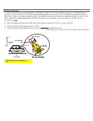
and Childs [18]. Figure 9 shows a schematic view of the bearing configuration and coordinate 

9 A set of slides follows this lecture notes – The slides show details and comparisons of (current) model predictions 

and test data in Refs. [12,13,18] 


system. Table 1 details the geometry of the pressure dam bearing, as detailed in Ref. [18]. Please 

note that Al-Jughaiman’s publication (including his M.s. thesis) misses details on the bearing 

geometry, lubricant inlet and feed conditions. Note that the pressure dam depth to clearance ratio 

and dam arc length relative to pad arc length follow standard best practices recommended by 

Nicholas and Allaire[19]. 

W 

Y 

X 

 

e 

Feed hole 

Pad with relief 

groove 

Pad with pressure dam 

170 deg 130 deg 

 

Figure 9. Schematic view of pressure dam bearing with relief groove. 

In the experiments, ISO VG 32 lubricant fills the thin film lands of the pressure dam bearing. 

An air turbine drives the test rigid shaft supported on ball bearings. The test bearing floats on the 

rotating shaft. The tester includes a hydraulic cylinder for static loading, and stinger connections 

to hydraulic shakers that excite the floating test bearing. The instrumentation includes load cells 

attached to the shaker stingers, eddy current sensors mounted on the bearing and facing the shaft, 

and accelerometers attached to the bearing housing. The parameter identification method is 


ased on frequency domain measurements and extracts the force coefficients from curve fits of 

the real and imaginary parts of the test system impedances. 

The maximum load (W) applied equals 12 kN (2,700 lb) which gives a specific pressure 

(W/LD) = 13.45 bar (~ 200 psi). 

Table 1. Dimensions and operating conditions of pressure dam bearing with relief groove 

tested by Jughaiman and Childs [18] 

Journal diameter D 117.1 mm 

Bearing Length L 76.2 mm 

Radial clearance c 0.142 mm 

pad arc 170 deg 

Dam arc length D 130 deg 

width (0.75 L) L D 57.1 mm 

depth 0.4 mm 

Reilef groove width L R 19.05 mm 

depth 0.1 mm 

Lubricant ISO VG 32 

Density 860 kg/m3 

Specific Heat Cp 2000 J/kg-C 

Thermal conductivity 0.13 W/m-C 

Viscosity at 45 C 0.028 Pa.s 

Visc-temp coefficient 0.034 1/C 

Inlet oil temperature 40-55 ? C 

Inlet oil pressure N/A bar 

Load range 0.1-12 kN 

Speed range 

4,6,8,10,12 krpm 

Closure 

Sept 2009: Lecture notes not yet complete. See slide presentation attached. 

Nomenclature 

c 

Nominal film (pad) clearance [m] 

c m 

bearing assembled clearance [m] 

C v 

Lubricant specific heat [J/kg-K] 

C Bearing damping force coefficients; 

Ns 

, = X, Y m 

D 

Journal diameter [m] 


e X , e Y Journal center eccentric displacements [m] 

F X , F Y Fluid film bearing reaction forces [N]; 

F S , F in , F up , Mass flow rates: supply, inlet to pad and upstream pad [kg/s] 

h 

Pad film thickness, c – r P cos(- P ) + e X cos() + e Y sin() [m] 

h X , h Y cos(), sin() 

h , h Heat transfer convection coefficients [W/m-K] 

B 

J 

K Bearing stiffness force coefficients; 

N , = X, Y m 

L 

Journal bearing axial length [m] 

M Added mass (fluid inertia) coefficients; 

N , = X, Y m 

n pe 

N em 

Q s 

Number of nodes per finite element 

Number of elements in flow domain 

heat flow conducted into bearing and journal surfaces [W/m] 

P 

Film pressure [Pa] 

P a 

Ambient pressure [Pa] 

P cav Lubricant cavitation pressure [Pa] 

P S 

Supply pressure [Pa] 

P 0 

Zeroth-order (aquilibrium) pressure [Pa] 

P First-order complex pressure fields; , = X, Y [Pa/m] 

q 

Volumetric flow rate per unit length [m 2 /s] 

R 

½ D. Journal radius, [m] 

2 

 

Re 

h 

 

s . Local squeeze film Reynolds number. 

 

r p 

(c-c m ). Pad preload [m] 

S Mechanical energy dissipation per unit area [W/m 2 ] 

t 

Time [s] 

T 

Lubricant mean flow temperature [degK] 

T S 

Supply temperature [degK] 

U, W Lubricant bulk-flow velocities, circumferential and axial [m/s] 

2 2 

W X , W Y Componentsof applied static load, W WX 

WY 

(x= R, y, z) Coordinate system on plane of bearing (starts at -X) 

(X, Y) Inertial coordinate system 

2 

Z Impedance force coefficients; K 

M i C 

, 

N , = X, Y m 

α v 

Viscosity-temperature coefficient [1/K] 

Δe X , Δe Y Dynamic displacements of journal center [m] 

x R . Circumferential coordinate [rad], 

l , t , p Arc pad leading and trailing edges, angle of min. film thickness (offset angle) 

[rad] 

v 

 

T TS 

 

S e 

. Fluid viscosity [Pa-s] 

e 

Element boundary 

ρ Fluid density [kg/m 3 ] 

 

Journal attitude angle with respect to static load vector [] 

 

i 

 

n pe 

1 

Finite element shape functions 


Rotor rotating speed, 

whirl frequency 

rad 

s 

e Finite element sub-domain 

Subscripts 

S 

in 

n,e,w,s 

N,W,E,S 

Superscripts 

e 

Supply condition 

Inlet to pad 

north, east, west and south of control volume 

North, east, west and south nodes 

element 

APPENDIX A. MODELS FOR HEAT CONVECTION COEFFICIENTS 

Reproduced from Ref.[7] 

The Reynolds-Colburn analogy between fluid friction and heat transfer for fully-developed 

flow determines the heat convection coefficients to accounting for heat flux from the fluid film 

into the shaft outer surface and from the film into the bearing cartridge. Over the entire 

laminar/turbulent boundary the Fanning friction factor f is: 

2/3 f 

Str 

(A.1) 

2 

where St 

h 

is the Stanton number, ρ and C v are the fluid density and specific heat, and U 

CU 

v 

cp 

 

is a mean flow velocity r 

is the Prandtl number, and and are fluid heat conduction 

 

coefficient and viscosity, respectively. 

From Eq. (A.1), heat convection coefficients h for laminar flow are derived from the Nusselt 

number; 

while for turbulent flow conditions 

where 4 area 

D hyd 

 

wetted perimeter 

is a hydraulic diameter. 

ch 1/3 

Nu 3 r 

 

(A.2) 

Dhydh 

0.8 0.4 

Nu 0.023Re 

 

r 

 

(A.3) 


References 

[1] Boncompain, R., Fillon M., and Frene, J., 1986, "Analysis of Thermal Effects in 

Hydrodynamic Bearings", ASME Journal of Tribology, 108 (2), pp. 219-224. 

[2] Kucinschi, B., ., Fillon M., Pascovici, M., and Frene, J., 2000, “A Transient 

Thermoelastohydrodynamic Study of Steadily Loaded Plain Journal Bearings using Finite 

Element Method Analysis", ASME Journal of Tribology, 122, (1), pp. 219-226, 2000. 

[3] Reinhart, F., and Lund, J. W., 1975, "The Influence of Fluid Inertia on the Dynamic 

Properties of Journal Bearings." ASME J. Lubrication Technology, 97, pp 154-167. 

[4] Smith, D. L., 1975, “Journal Bearing Dynamic Characteristics-Effect of Inertia of Lubricant, 

Proc. Inst. Mech. Engrs., Paper No. 21, 179, Pt.3J, pp 37-44. 

[5] San Andrés, L., and Vance, J., 1987, "Effect of Fluid Inertia on Squeeze Film Damper Forces 

for Small Amplitude Circular Centered Motions," ASLE Transactions, 30, No. 1, pp. 69-76. 

[6] San Andrés, L., 2009, Modern Hydrodynamic Lubrication Theory, Notes 10: 

Thermohydrodynamic Bulk-Flow Model in Thin Film Lubrication, Texas A&M University, 

http://phn.tamu.edu/me626 [Accessed April 2009] 

[7] San Andrés, L., Yang, Z. and Childs, D., 1993, "Thermal Effects in Cryogenic Liquid 

Annular Seals, I: Theory and Approximate Solutions", ASME Journal of Tribology, 115, 2, 

pp. 267-276. 

[8] San Andrés, L., and Kerth, J., 2004, “Thermal Effects on the Performance of Floating Ring 

Bearings for Turbochargers”, Journal of Engineering Tribology, Special Issue on Thermal 

Effects on Fluid Film Lubrication, IMechE Proceedings Part J, 218, pp. 437-450. 

[9] San Andrés, L., 2009, Modern Hydrodynamic Lubrication Theory, Notes 6: Cavitation in 

Liquid Film Bearings, Texas A&M University, http://phn.tamu.edu/me626 [Accessed 

September 2009] 

[10] Pinkus, O., 1990, “Thermal Aspects of Fluid Film Tribology,” ASME Press, N.Y. 

[11] Lund, J. W., and E.B. Arwas, 1964, “A Simultaneous Solution of the Lubrication and the 

Energy Equations for Turbulent Journal Bearing Films,” MTI Report N o 64-TR-31, MTI, Inc., 

N.Y. 

[12] Ferron, J., Frene, J., and R. Boncompain, 1983, “A Study of the Thermohydrodynamic 

Performance of a Plain Journal Bearing Comparison between Theory and Experiments”, 

ASME Journal of Tribology, Vol. 105, pp. 422-428, 

[13] Brito, F.P., Miranda, A.S., Bouter, J., and Fillon, M., Frene, J., and R. Boncompain, 2007, 

“Experimental investigation on the influence of Supply temperature and Supply Pressure on 

the Performance of a Two-Axial Groove Hydrodynamic Journal Bearing”, ASME Journal of 

Tribology, Vol. 129, pp. 98-105. 

[14] Lund, J., 1987, “Review of the Concept of Dynamic Coefficients for Fluid Film Journal 

Bearings,” ASME Journal of Tribology, Vol. 109, pp. 37- 41. 

[15] Klit, P. and Lund, J. W., 1988, “Calculation of the Dynamic Coefficients of a Journal 

Bearing Using a Variational Approach,” ASME Journal of Tribology, Vol. 108, pp. 421 - 425. 


[16] Reddy J. N., Gartling, D. K., 2001, The Finite Element Method in Heat transfer and Fluid 

Dynamics, CRC Press, Florida, Chap. 2. 

[17] Patankar, S.V., 1980, Numerical Heat Transfer and Fluid Flow, Hemisphere Pubs, N.Y. 

[18] Al-Jughaiman, and Childs, D., 2007, “Static and Dynamic Characteristics for a Pressure- 

Dam Bearing”, ASME Paper GT2007-25577. 

[19] Nicholas, J., and Allaire, P., 1980, “Analysis of Step Journal Bearings-Finite Length and 

Stability,” ASLE Transactions, 22, pp. 197-207. 

Additional (numerical analyses) references 

The references below detail numerical analyses for hydrodynamic and hydrostatic liquid and gas 

bearings, rigid pads and tilting pads. Note that tilting pad bearings show frequency dependent 

force coefficients. The same holds true for gas bearings 

Tilting Pad (liquid) bearings 

San Andrés, L., "Turbulent Flow, Flexure-Pivot Hybrid Bearings for Cryogenic Applications," 

ASME Journal of Tribology, Vol. 118, 1, pp. 190-200, 1996 

Gas bearings 

San Andrés, L., 2006, “Hybrid Flexure Pivot-Tilting Pad Gas Bearings: Analysis and 

Experimental Validation,” ASME Journal of Tribology, 128, pp. 551-558. 

Delgado, A., L., San Andrés, and J. Justak, 2004, “Analysis of Performance and Rotordynamic 

Force Coefficients of Brush Seals with Reverse Rotation Ability”, ASME Paper GT 2004- 

53614 

San Andrés, L., and D. Wilde, 2001, “Finite Element Analysis of Gas Bearings for Oil-Free 

Turbomachinery,” Revue Européenne des Eléments Finis, 10 (6/7), pp. 769-790. 

Zirkelback, N., and L. San Andrés, 1999, "Effect of Frequency Excitation on the Force 

Coefficients of Spiral Groove Thrust Bearings and Face Gas Seals,” ASME Journal of 

Tribology, 121(4), pp. 853-863. 

Foil Gas bearings 

San Andrés, L., and Kim, T.H., “Thermohydrodynamic Analysis of Bump Type gas Foil 

Bearings: A Model Anchored to Test Data” GT2009-59919 

San Andrés, L., and Kim, T.H., 2009, “Analysis of Gas Foil Bearings Integrating FE Top Foil 

Models,” Tribology International, 42(2009), pp. 111-120. 

Kim, T.H., and L. San Andrés, 2008, “Heavily Loaded Gas Foil Bearings: a Model Anchored to 

Test Data,” ASME Journal of Engineering for Gas Turbines and Power, Vol. 130(1), pp. 

012504-1-8. (ASME Paper GT 2005-68486). 

Kim, T.H., and L. San Andrés, 2006, “Limits for High Speed Operation of Gas Foil Bearings,” 

ASME Journal of Tribology, 128, pp. 670-673 

San Andrés, L., 1995, "Turbulent Flow Foil Bearings for Cryogenic Applications," ASME 

Journal of Tribology, 117(1), pp. 185-195. 


Hydrostatic/hydrodynamic liquid bearings and seals 

San Andrés, L., "Thermohydrodynamic Analysis of Fluid Film Bearings for Cryogenic 

Applications," AIAA Journal of Propulsion and Power, Vol. 11, 5, pp. 964-972, 1995. 

Yang, Z., San Andrés, L. and Childs, D., "Thermal Effects in Cryogenic Liquid Annular Seals, 

II: Numerical Solution and Results", ASME Journal of Tribology, Vol. 115, 2, pp. 277-284, 

1993 (ASME Paper 92-TRIB-5). 

San Andrés, L., Yang, Z. and Childs, D., "Thermal Effects in Cryogenic Liquid Annular Seals, I: 

Theory and Approximate Solutions", ASME Journal of Tribology, Vol. 115, 2, pp. 267-276, 

1993 (ASME Paper 92-TRIB-4). 

San Andrés, L., "Analysis of Turbulent Hydrostatic Bearings with a Barotropic Fluid," ASME 

Journal of Tribology, Vol. 114, 4,pp. 755-765,1992. 

San Andrés, L., "Fluid Compressibility Effects on the Dynamic Response of Hydrostatic Journal 

Bearings," WEAR, Vol. 146, pp. 269-283, 1991 

San Andrés, L., "Turbulent Hybrid Bearings with Fluid Inertia Effects", ASME Journal of 

Tribology, Vol. 112, pp. 699-707, 


Computational code 

Fortran code : complete – including prediction of inertia force 

coefficients 

GUI (Excel interface) –complete 

Examples for calibration: 

(pressure and temperature fields) 

oil 360 deg journal bearing 

Dowson et al. (1966) 

Ferron, Frene, Boncompain (1983) 

Costa, Fillon (2000 2003) 

oil two groove journal bearing 

Costa, Fillon (2000 2003) 

Brito, Fillon (2006, 2007) 

Pressure dam bearing 

Childs et al (2007, 2008) 

Load capacity & force 

coefficients 

19

Example 1 : Ferron bearing (1983) 

Journal diameter D 100 mm 

Bearing Length L 80 mm 


Groove width 

mm 

groove arc length 18 deg 

Lubricant 






Inlet oil temperature 40 C 

Inlet oil pressure 0.7 bar 

Load range 

1kN-10 kN 

Speed range 

1-4 kRPM 

Prandtl No 426 

Load No 23.98 

Diffusivity 

7.55814E-08 m2/s 

Ferron,J., Frene, J., and R. 

Boncompain, 1983, “A Study 

of the Thermohydrodynamic 

Performance of a Plain 

Journal Bearing Comparison 

Between Theory and 

Experiments”, ASME 

Journal of Tribology, Vol. 

105, pp. 422-428, 

flow 

 

W 

Y 

X 

Sommerfeld # 

S 

 

 

N L D 

W 

 

 

 

R 

C 

2 

 

 

 

20

Ferron et al. bearing (1983) 

Load 

Test data 

50 

Film temperature 

temperature 

Temperature (deg C) 

48 

46 

44 

42 

40 

0 30 60 90 120 150 180 210 240 270 300 330 360 

* 

angle (deg) 

2 

Midplane pressure pressure 

Pressure (MPa) 

1.5 

1 

0.5 

0 

0 30 60 90 120 150 180 210 240 270 300 330 360 

* 

angle (deg) 

p 

* 

Pressure and temperature fields – 4 kRPM, 6 kN 

21


Load 

Test data 

eccentricity ratio 

0.9 

0.8 

0.7 

0.6 

0.5 

0.4 

0.3 

0.2 

2000 

3000 

4000 

RPM 

0.1 

Eccentricity ratio (e/c) vs Sommerfeld # 

0.0 

0.0 0.1 0.2 0.3 0.4 0.5 0.6 0.7 0.8 0.9 

2 

N L D R 

2 

Sommerfeld # S 

W NLD C R 

S 

 

 

W C 

22


Load 

Test data 

0.9 

0.8 

eccentricity ratio (e/c) 

0.7 

0.6 

0.5 

0.4 

0.3 

0.2 

2 krpm 

0.1 

3 krpm kRPM 

4 krpm 

0.0 

0.0 2.0 4.0 6.0 8.0 10.0 12.0 

Load (kN) 

Journal eccentricity (e/c) vs. applied static load 

23


Load 

Test data 

45 

40 

35 

2000 

3000 

4000 

RPM 

Peak pressure 

30 

25 

20 

15 

10 

5 

0 

0.0 0.1 0.2 0.3 0.4 0.5 0.6 0.7 0.8 0.9 


Peak film pressure vs. eccentricity ratio (e/c) 

24


Load 

14 

12 

deg C 

Test data 

Peak temperature rise 

10 

8 

6 

4 

2 

Tsupply=40 C 

2000 

3000 

4000 RPM 

0 

0.0 0.1 0.2 0.3 0.4 0.5 0.6 0.7 0.8 0.9 


Peak film temperature vs. eccentricity ratio (e/c) 

25

Example 2: two axial groove bearing 

Journal diameter D 100 mm 

Bearing Length L 80 mm 


preload r p 0 mm 

Feed groove width 70 mm 

Pad arc length 162 deg 

Lubricant 






Inlet oil temperature 35,40,50 C 

Inlet oil pressure 

0.7,1.4, 2.1 bar 

Load range 

1kN-10 kN 

Speed range 

1-4 kRPM 

Prandtl No 451 

Brito,F.P., Miranda, A.S., Bouter, J., 

and Fillon, M., Frene, J., and R. 

Boncompain, 2007, “Experimental 

investigation on the influence of 

Supply temperature and Supply 

Pressure on the Performance of a 

Two-Axial Groove Hydrodynamic 

Journal Bearing”, ASME Journal of 

Tribology, Vol. 129, pp. 98-105, 

Y 

W 

Top pad 

flow 

X 

bottom pad 

26

Brito et al. bearing (2007) 

Midplane pressure 

Film temperature 

Journal locus 

Load 

Test data 

Predictions 

e/c=0.43 

56 deg 

1.35 kW 

3.0 LPM 

28 bar max 

Pressure (MPa) 

3.5 

3 

2.5 

2 

1.5 

1 

0.5 

temperature (C) 

temperature (C) 

70 

65 

60 

55 

50 

45 

0 

40 

0 45 90 135 180 225 270 315 360 

0 45 90 135 180 225 270 315 360 

* angle (deg) 

angle (deg) 

* 

Pressure and temperature fields – 4 kRPM, 10 kN 

27

Example 3 – Pressure dam bearing 

Journal diameter D 117.1 mm 

Bearing Length L 76.2 mm 


pad arc 170 deg 

Dam arc length D 130 deg 

width (0.75 L) L D 57.1 mm 

depth 0.4 mm 

Reilef groove width L R 19.05 mm 

depth 0.1 mm 

Lubricant ISO VG 32 






Inlet oil temperature 40-55 ? C 

Inlet oil pressure N/A bar 

Load range 0.1-12 kN 

Speed range 

4,6,8,10,12 krpm 

Al-Jughaiman, and Childs, D., 2007, 

“Static and Dynamic Characteristics 

for a Pressure-Dam Bearing”, ASME 

Paper GT2007-25577 

e 

Y 

W 

X 

Missing details on bearing geometry, lubricant and feed conditions. Even with test 

data at hand, not able to reproduce test results in paper. VERY PECULIAR 28 

THERMAL EFFECTS


12 

10 

Power Loss (kW) 

8 

6 

4 

2 

0 

0 250 500 750 1000 1250 1500 

Unit Load (kPa) 

GT2007-25577 Power loss 

4000 rpm 

6000 rpm 

8000 rpm 

10000 rpm 

12000 rpm 

29


TAMU Pressure Dam Bearing with relief track 

1.0 

145 psi 

eccentricity ratio (e/c) 

0.9 

0.8 

0.7 

0.6 

0.5 

0.4 

0.3 

0.2 

0.1 

0.0 

e 

Y 

W 

X 

0 200 400 600 800 1000 1200 1400 

Unit Load (W/LD) [kPa] 

4 krpm (pred) 

10 krpm (pred) 

4 krpm (test data) 

10 krpm (test data) 


test data 12 krpm 

Journal eccentricity vs specific pressure 

30


TAMU Pressure Dam Bearing 

Attitude angle (deg) 

90 

80 

70 

60 

50 

40 

30 

20 

10 

0 

4 krpm (pred) 


4 krpm (test) 

10 krpm (test) 

0 200 400 600 800 1000 1200 1400 

e 

145 psi 

Y 

W 

X 


Attitude angle vs specific pressure 

31



Y 

W 

Stiffness [MN/m] 

1200 

1000 

800 

600 

400 

200 

0 

KYY 

4 krpm (pred) 


test 4 krpm 

test 10 krpm 

0 200 400 600 800 10001451200 psi 1400 

e 

X 


Direct stiffness KYY vs specific pressure 

32



250 

145 psi 

Y 

W 

X 

200 

KXX 

e 


150 

100 

50 

0 

4 krpm (pred) 


4 krpm (test) 

10 krpm (test) 

0 200 400 600 800 1000 1200 1400 


Direct stiffness K XX vs specific pressure 

33



TAMU Pressure Dam Bearing with relief track 

180 

160 

140 

120 

100 

80 

60 

40 

20 

0 

-20 

KXY 

4 krpm (pred) 


test 4 krpm 

test 10 krpm 

145 psi 

0 200 400 600 800 1000 1200 1400 

e 

Y 

W 

X 


Cross stiffness K XY vs specific pressure 

34



Note: prediction changed sign 

Y 

W 

600 

145 psi 

e 

X 

500 

KYX 


400 

300 

200 

100 

0 

4 krpm (pred) 


test 4 krpm 

test 10 krpm 

0 200 400 600 800 1000 1200 1400 


Cross stiffness K YX vs specific pressure 

35


Damping [kN.s/m] 


2000 

1800 

1600 

1400 

1200 

1000 

800 

600 

400 

CYY 

4 krpm (pred) 


test 4 krpm 

test 10 krpm 

e 

Y 

W 

X 

200 

0 

145 psi 

0 200 400 600 800 1000 1200 1400 


Direct DAMPING C YY vs specific pressure 

36



300 

145 psi 

Y 

W 

X 

250 

CXX 

e 


200 

150 

100 

50 

0 

4 krpm (pred) 


test 4 krpm 

test 10 krpm 

0 200 400 600 800 1000 1200 1400 


Direct DAMPING C XX vs specific pressure 

37



600 

500 

CXY 

4 krpm (pred) 


test 4 krpm 

test 10 krpm 

e 

Y 

W 

X 


400 

300 

200 

100 

0 

145 psi 

0 200 400 600 800 1000 1200 1400 


Cross DAMPING C XY vs specific pressure 

38




700 

600 

500 

400 

300 

200 

100 

CYX 

Note: prediction changed sign 

4 krpm (pred) 


test 4 krpm 

test 10 krpm 

e 

Y 

W 

X 

0 

145 psi 

0 200 400 600 800 1000 1200 1400 


Cross DAMPING C YX vs specific pressure 

39


Whirl frequency ratio 


0.50 

0.45 

0.40 

0.35 

0.30 

0.25 

0.20 

0.15 

0.10 

WFR 

4 krpm (pred) 


e 

Y 

W 

X 

0.05 

0.00 

0 200 400 600 800 1000 1200 1400 


Whirl frequency ratio WFR vs specific pressure 

40


kg 

Inertia coefficients 

50.0 

45.0 

40.0 

35.0 

30.0 

25.0 

20.0 

15.0 

10.0 

5.0 

0.0 

-5.0 

0 200 400 600 800 1000 1200 1400 1600 

Unit Load [kPa] 

Mxx 

Myy 

Mxy 

Myx 

10 krpm 

Added Mass Coefficients WFR vs specific pressure 

41

Thermal analysis of finite length journal bearings including fluid inertia

Create successful ePaper yourself

Delete template?

Save as template?