Non-linear Least- Squares Fitting with MPFIT - UGAstro
Non-linear Least- Squares Fitting with MPFIT - UGAstro
Non-linear Least- Squares Fitting with MPFIT - UGAstro

Create successful ePaper yourself
Turn your PDF publications into a flip-book with our unique Google optimized e-Paper software.
<strong>Non</strong>-<strong>linear</strong> <strong>Least</strong>-<br />
<strong>Squares</strong> <strong>Fitting</strong> <strong>with</strong><br />
<strong>MPFIT</strong><br />
Some documentation:<br />
http://www.physics.wisc.edu/~craigm/idl/fitting.html<br />
Tutorial:<br />
http://www.physics.wisc.edu/~craigm/idl/mpfittut.html
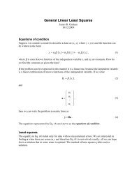
<strong>Non</strong>-<strong>linear</strong> problems must be solved iteratively--<br />
unlike the problems you’ve used least-squares on<br />
before this lab.<br />
<strong>Fitting</strong> a Gaussian<br />
function to data is a<br />
classic example.<br />
f (x,µ,σ) = 1<br />
σ √ 2π e−(x−µ)2 /2σ 2<br />
Can’t use <strong>linear</strong><br />
techniques on this<br />
problem.
<strong>MPFIT</strong> example:<br />
<strong>Fitting</strong> a Gaussian<br />
You have:<br />
- X values<br />
- Y values<br />
- Y errors<br />
(assume x values have<br />
no error in this<br />
example)<br />
Step 1: Gather your data.
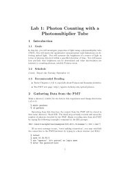
<strong>MPFIT</strong> example:<br />
<strong>Fitting</strong> a Gaussian<br />
Step 2: Choose your model.<br />
Ours will be a Gaussian<br />
function plus a constant offset.<br />
This has four parameters:<br />
a0 = value at peak<br />
a1 = central x value<br />
a2 = sigma<br />
a3 = offset<br />
a3<br />
a0<br />
a2<br />
a1
<strong>MPFIT</strong> example:<br />
<strong>Fitting</strong> a Gaussian<br />
Step 3: Make a function that returns the difference<br />
between your data and your model, weighted by<br />
the errors on the data<br />
function mygaussian, p, x=x, y=y, err=err<br />
; p = [a0, a1, a2, a3]<br />
model = p[3] + p[0] * exp(-0.5 * ((x-p[1])/p[2])^2.)<br />
return, (y-model)/err<br />
end
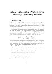
<strong>MPFIT</strong> example:<br />
<strong>Fitting</strong> a Gaussian<br />
Step 3: Pick an initial guess for the parameters p<br />
guessp = [900., 2., 1., 1000.]<br />
Try to make a good guess,<br />
some problems can be<br />
sensitive to the initial guess.<br />
(This can be automated).<br />
a3<br />
a0<br />
a2<br />
a1
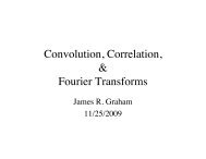
<strong>MPFIT</strong> example:<br />
<strong>Fitting</strong> a Gaussian<br />
Step 4: Use <strong>MPFIT</strong><br />
guessp = [950., 2.5, 1., 1000.]<br />
fa = {X:x, Y:y, ERR:err}<br />
p = mpfit(‘mygaussian’, guessp, functargs=fa)<br />
mpfit doesn’t care about your data except in how it<br />
deviates from the model, so everything data-related is<br />
packaged up in “fa” the function arguments structure
IDL> p = mpfit('mygaussian', guessp, functargs=fa)<br />
Iter 1 CHI-SQUARE = 1462.3943<br />
DOF = 196<br />
P(0) = 950.000<br />
P(1) = 2.50000<br />
P(2) = 1.00000<br />
P(3) = 1000.00<br />
Iter 2 CHI-SQUARE = 353.66009<br />
DOF = 196<br />
P(0) = 749.300<br />
P(1) = 2.26459<br />
P(2) = 1.39788<br />
P(3) = 1007.73<br />
Iter 8 CHI-SQUARE = 187.48896<br />
DOF = 196<br />
P(0) = 837.138<br />
P(1) = 2.15507<br />
P(2) = 1.44884<br />
P(3) = 997.619
Other things you can do <strong>with</strong> <strong>MPFIT</strong><br />
- adjust the weighting of each point<br />
- limit parameters to be <strong>with</strong>in a certain range<br />
- hold some parameters constant<br />
- adjust step sizes and convergence criteria<br />
- lots of other stuff, very powerful!
Trying it out! (these programs are on the website)<br />
- use fakedata.sav, mygaussian.pro and testgaussfit.pro<br />
to see how mpfit works in the case I’ve outlined in this<br />
presentation<br />
- use makecircdata.pro, mycirc.pro and testcircfit.pro<br />
to see how mpfit works in the case where you have<br />
one independent variable (like time) and two<br />
dependent variables (like RA and Dec)