Fourier transforms & the convolution theorem - UGAstro

Convolution, Correlation,
&
Fourier Transforms
James R. Graham
11/25/2009

Introduction
• A large class of signal processing
techniques fall under the category of
Fourier transform methods
– These methods fall into two broad categories
• Efficient method for accomplishing common data
manipulations
• Problems related to the Fourier transform or the
power spectrum

Time & Frequency Domains
• A physical process can be described in two ways
– In the time domain, by h as a function of time t, that is
h(t), -∞ < t < ∞
– In the frequency domain, by H that gives its amplitude
and phase as a function of frequency f, that is H(f), with
-∞ < f < ∞
• In general h and H are complex numbers
• It is useful to think of h(t) and H(f) as two
different representations of the same function
– One goes back and forth between these two
representations by Fourier transforms

Fourier Transforms
∞
∫
−∞
H( f )= h(t)e −2πift dt
h(t)=
∞
∫
−∞
H ( f )e 2πift df
• If t is measured in seconds, then f is in cycles per
second or Hz
• Other units
– E.g, if h=h(x) and x is in meters, then H is a function of
spatial frequency measured in cycles per meter

Fourier Transforms
• The Fourier transform is a linear operator
– The transform of the sum of two functions is
the sum of the transforms
h 12
= h 1
+ h 2
H 12
( f )=
∞
∫
−∞
∞
h 12
e −2πift dt
= ∫ ( h 1
+ h 2 )e −2πift dt = ∫ h 1
e −2πift dt + h 2
e −2πift dt
−∞
= H 1
+ H 2
∞
−∞
∞
∫
−∞

Fourier Transforms
• h(t) may have some special properties
– Real, imaginary
– Even: h(t) = h(-t)
– Odd: h(t) = -h(-t)
• In the frequency domain these symmetries
lead to relations between H(f) and H(-f)

FT Symmetries
If…
h(t) real
h(t) imaginary
h(t) even
h(t) odd
h(t) real & even
h(t) real & odd
h(t) imaginary & even
h(t) imaginary & odd
Then…
H(-f) = [ H(f) ] *
H(-f) = -[ H(f) ] *
H(-f) = H(f) (even)
H(-f) = - H(f) (odd)
H(f) real & even
H(f) imaginary & odd
H(f) imaginary & even
H(f) real & odd

Elementary Properties of FT
h(t)↔ H ( f )
h(at)↔ 1 a H ( f /a)
h(t − t 0
)↔ H ( f )e −2πift 0
Fourier Pair
Time scaling
Time shifting

Convolution
• With two functions h(t) and g(t), and their
corresponding Fourier transforms H(f) and
G(f), we can form two special combinations
– The convolution, denoted f = g * h, defined by
( ) = g ∗ h ≡ g(τ )h(t −
f t
∞
∫
−∞
τ )dτ

Convolution
• g*h is a function of time, and
g*h = h*g
– The convolution is one member of a transform pair
g∗ h ↔ G( f )H( f )
• The Fourier transform of the convolution is the
product of the two Fourier transforms!
– This is the Convolution Theorem

Correlation
• The correlation of g and h
Corr(g,h) ≡
∞
∫
−∞
g(τ + t)h(τ )dτ
• The correlation is a function of t, which is
known as the lag
– The correlation lies in the time domain

Correlation
• The correlation is one member of the transform
pair
Corr(g,h) ↔ G( f )H * ( f )
– More generally, the RHS of the pair is G(f)H(-f)
– Usually g & h are real, so H(-f) = H*(f)
• Multiplying the FT of one function by the
complex conjugate of the FT of the other gives the
FT of their correlation
– This is the Correlation Theorem

Autocorrelation
• The correlation of a function with itself is
called its autocorrelation.
– In this case the correlation theorem becomes
the transform pair
Corr(g,g) ↔ G( f )G * ( f ) = G( f ) 2
– This is the Wiener-Khinchin Theorem

Convolution
• Mathematically the convolution of r(t) and
s(t), denoted r*s=s*r
• In most applications r and s have quite
different meanings
– s(t) is typically a signal or data stream, which
goes on indefinitely in time
– r(t) is a response function, typically a peaked
and that falls to zero in both directions from its
maximum

The Response Function
• The effect of convolution is to smear the
signal s(t) in time according to the recipe
provided by the response function r(t)
• A spike or delta-function of unit area in s
which occurs at some time t 0 is
– Smeared into the shape of the response function
– Translated from time 0 to time t 0 as r(t - t 0 )

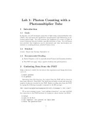
Convolution
s(t)
r(t)
s*r
• The signal s(t) is convolved with a response function r(t)
– Since the response function is broader than some features in the
original signal, these are smoothed out in the convolution

Fourier Transforms & FFT
• Fourier methods have revolutionized many fields
of science & engineering
– Radio astronomy, medical imaging, & seismology
• The wide application of Fourier methods is due to
the existence of the fast Fourier transform (FFT)
• The FFT permits rapid computation of the discrete
Fourier transform
• Among the most direct applications of the FFT are
to the convolution, correlation & autocorrelation
of data

The FFT & Convolution
• The convolution of two functions is defined for
the continuous case
– The convolution theorem says that the Fourier
transform of the convolution of two functions is equal
to the product of their individual Fourier transforms
g∗ h ↔ G( f )H( f )
• We want to deal with the discrete case
– How does this work in the context of convolution?

Discrete Convolution
• In the discrete case s(t) is represented by its
sampled values at equal time intervals s j
• The response function is also a discrete set r k
– r 0 tells what multiple of the input signal in channel j is
copied into the output channel j
– r 1 tells what multiple of input signal j is copied into the
output channel j+1
– r -1 tells the multiple of input signal j is copied into the
output channel j-1
– Repeat for all values of k

Discrete Convolution
• Symbolically the discrete convolution is
with a response function of finite duration,
N, is
N / 2
∑
k=−N / 2 +1
( s∗ r) = s r j k j−k
( s∗ r) ↔S R j l l

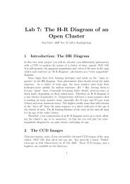
Discrete Convolution
s j
r k
(s*r) j
• Convolution of discretely sampled functions
– Note the response function for negative times wraps
around and is stored at the end of the array r k

Examples
• Java applet demonstrations
– Continuous convolution
• http://www.jhu.edu/~signals/convolve/
– Discrete convolution
• http://www.jhu.edu/~signals/discreteconv/

Suppose that f and g are functions of time
f (t) =
∞
∫ F(ν) e 2πiνt dν and g(t)= ∫ G(ν) e 2πiνt dν
-∞
The convolution f*g says
f ∗ g =
∫
∞
-∞
g(t ') f (t − t ') dt '
∞
∞
= ∫
2πiν (t −t ')
g(t ') ⎡ ∫ F(ν) e dν ⎤dt '
-∞ ⎣⎢ -∞
⎦⎥
Swap the order of integration
∞
∞
= ∫ F(ν) ⎡
∫ g(t ') e −2πiνt ' dt ' ⎤e -∞ ⎣⎢ -∞
⎦⎥
2πiνt dν
= FT F(ν)G(ν)
Voila!
[ ]
∞
-∞