General linear least squares - UGAstro

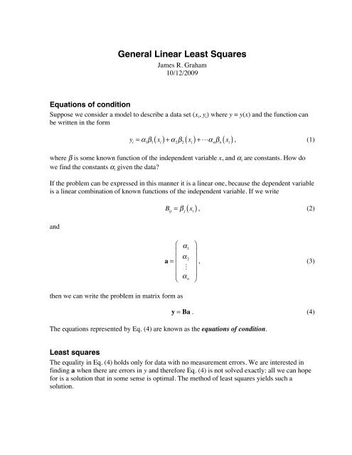
General Linear Least SquaresJames R. Graham10/12/2009Equations of conditionSuppose we consider a model to describe a data set (x i , y i ) where y = y(x) and the function canbe written in the formy i= α 1β 1( x i ) + α 2β 2x i( ) +α nβ nx i( ), (1)where β is some known function of the independent variable x, and α i are constants. How dowe find the constants α i given the data?If the problem can be expressed in this manner it is a linear one, because the dependent variableis a linear combination of known functions of the independent variable. If we writeandB ij= β j⎛⎜a = ⎜⎜⎜⎝then we can write the problem in matrix form asα 1α 2α n( ) , (2)x i⎞⎟⎟ , (3)⎟⎟⎠y = Ba . (4)The equations represented by Eq. (4) are known as the equations of condition.Least squaresThe equality in Eq. (4) holds only for data with no measurement errors. We are interested infinding a when there are errors in y and therefore Eq. (4) is not solved exactly: all we can hopefor is a solution that in some sense is optimal. The method of least squares yields such asolution.

We can write a compact expression for the sum of the squares of the residuals,χ 2 = y − Ba 22, (5)where the notation ||…|| 2 is used to denote the Euclidian vector norm 1 ,x 2 2= x T 2x = ∑ x i, (6)and the superscript T denotes the transpose. Expanding Eq. (5) we findiχ 2 = ( y − Ba) T ( y − Ba)= y T y − 2y T Ba + a T B T Ba.(7)We want to minimize this expression as a function of a, so that the first derivatives with respectto a are zeroor∂χ 2∂a = −2BT y + 2B T Ba = 0 , (8)B T Ba = B T y . (9)Thus, the unknown vector a is found by multiplying each side by the inverse matrix (B T B) -1( B T B) −1 B T Ba = B T B( ) −1 B T y( ) −1 B T y.a = B T B(10)The quantity (B T B) -1 is known as the generalized or Moore-Penrose pseudo-inverse of B.Sophisticated versions of general least squares methods use singular value decomposition tocompute the inverse of B T B.1In two or three dimensions the Euclidian vector norm is just the magnitude (length) of thevector (think Pythagoras’ theorem).

An simple example: uniform acceleration from restSuppose we have a set of data described by a parabolic relationx = 1 2 gt 2 ,e.g., the distance traveled by a body dropped from rest. How do we find the value of g? Somedata are shown in Figure 1.Figure 1: Measurement of the position of a body falling from rest under gravity with g =9.81 m s -2 . The dotted line shows the fit that you get if you fit a general quadratic.If the data vectors are t and x, in IDL the solution is implemented as follows:b = transpose([0.5*t^2])y = transpose(x)psi = invert( transpose(b) ## b)ans = psi ## transpose( b) ## yNote that the transpose function in the first two steps is to convert the row vectors intocolumn vectors. In IDL the matrix multiplication operator is ##.The conventional (but wrong) approach would be to fit a second order polynomial to the data:res = poly_fit(t,x,2)

In the example in Figure 1, the parabolic fit gives g = 9.93 m s -2 , whereas the polynomial fitimplies that the initial position is -0.29 m, the initial velocity is 1.81 m s -1 and the accelerationis 6.18 m s -2 . Polynomial fitting fails to take account of our knowledge that the initial positionand velocity are zero, and as a consequence gives an inaccurate value for the acceleration.Example: Circular motionNow suppose our task is to determine the radius of a wheel by measuring the x-coordinate of apoint on the circumference as the wheel rotates at a known frequency ω. The position of thatpoint is given byx = x 0+ Rsin( ωt) .From measurements of (t, x) we want to find x 0 and R. For this example, the relevant fragmentof IDL code isb = transpose([[replicate(1.,npts)],[sin(omega*t)]])y = transpose(x)psi = invert( transpose(b) ## b)ans = psi ## transpose( b) ## yAn example of such a fit is shown in Figure 2.Figure 2: Time series of measurement of a point on the circumference of a wheel rotatingat known angular frequency ω. A linear least squares fit to x = x 0 + Rsin(ωt) yields theradius and the x-coordinate of the point of rotation.Note the limitation of this method—we cannot determine ω from the data; we have to know therotation rate. Problems where unknowns enter other than in linear combinations fall into thecategory of non-linear least squares. There are no closed-form solutions to non-linear

problems: they are solved using iterative methods that require an initial guess for the modelparameters.At first sight some problems appear non-linear, e.g., the case of the rotating wheel when thephase, φ, is unknownx = x 0+ Rsin( ωt + φ) .However, by use of trigonometric identities we can writewhich is a linear problem.x = x 0+ Rcos( φ )sin( ωt) + Rsin( φ )cos( ωt),