A steady state approach to calculation of valve pressure rise rate ...
A steady state approach to calculation of valve pressure rise rate ...
A steady state approach to calculation of valve pressure rise rate ...

You also want an ePaper? Increase the reach of your titles
YUMPU automatically turns print PDFs into web optimized ePapers that Google loves.
Konference ANSYS 2011<br />
A <strong>steady</strong> <strong>state</strong> <strong>approach</strong> <strong>to</strong> <strong>calculation</strong><br />
<strong>of</strong> <strong>valve</strong> <strong>pressure</strong> <strong>rise</strong> <strong>rate</strong> characteristics<br />
Ján Oravec<br />
Technical centre, Sauer-Danfoss a.s., Považská Bystrica<br />
joravec@sauer-danfoss.com<br />
Abstract: Pressure relief <strong>valve</strong>s are widely used in hydrostatic circuits. The <strong>pressure</strong> <strong>rise</strong> <strong>rate</strong> characteristics are<br />
one <strong>of</strong> the most important descriptions <strong>of</strong> the <strong>valve</strong>s performance. This article proposes design <strong>of</strong> the basic<br />
<strong>pressure</strong> <strong>rise</strong> <strong>rate</strong> characteristic <strong>of</strong> <strong>valve</strong> using only a few CFD <strong>calculation</strong>s. These <strong>calculation</strong>s are performed<br />
for several poppet strokes and flow values. The method is shown for charge <strong>pressure</strong> relief <strong>valve</strong> but can be used<br />
similarly for any poppet type <strong>valve</strong>.<br />
Keywords: <strong>pressure</strong> relief <strong>valve</strong>, hydrostatics, <strong>pressure</strong> <strong>rise</strong> <strong>rate</strong> characteristic, CFD<br />
1. Introduction<br />
Pressure relief <strong>valve</strong>s are essential components in hydrostatic systems. They protect the systems against<br />
excessive <strong>pressure</strong>s or maintain <strong>pressure</strong>s at desired levels. The performances <strong>of</strong> such <strong>valve</strong>s are represented by<br />
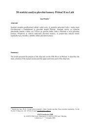
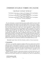
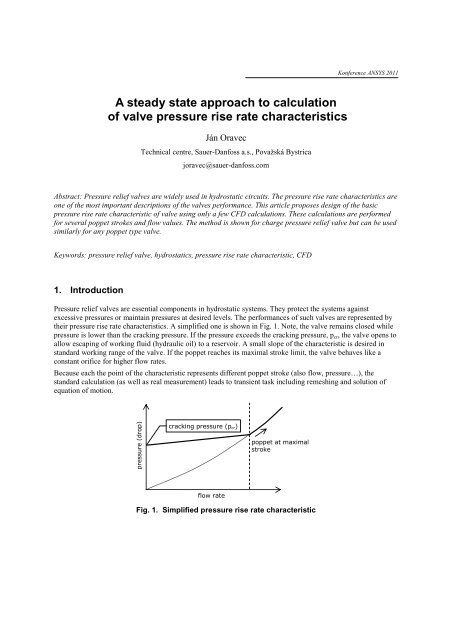
their <strong>pressure</strong> <strong>rise</strong> <strong>rate</strong> characteristics. A simplified one is shown in Fig. 1. Note, the <strong>valve</strong> remains closed while<br />
<strong>pressure</strong> is lower than the cracking <strong>pressure</strong>. If the <strong>pressure</strong> exceeds the cracking <strong>pressure</strong>, p cr , the <strong>valve</strong> opens <strong>to</strong><br />
allow escaping <strong>of</strong> working fluid (hydraulic oil) <strong>to</strong> a reservoir. A small slope <strong>of</strong> the characteristic is desired in<br />
standard working range <strong>of</strong> the <strong>valve</strong>. If the poppet reaches its maximal stroke limit, the <strong>valve</strong> behaves like a<br />
constant orifice for higher flow <strong>rate</strong>s.<br />
Because each the point <strong>of</strong> the characteristic represents different poppet stroke (also flow, <strong>pressure</strong>…), the<br />
standard <strong>calculation</strong> (as well as real measurement) leads <strong>to</strong> transient task including remeshing and solution <strong>of</strong><br />
equation <strong>of</strong> motion.<br />
<strong>pressure</strong> (drop)<br />
cracking <strong>pressure</strong> (p cr)<br />
poppet at maximal<br />
stroke<br />
flow <strong>rate</strong><br />
Fig. 1. Simplified <strong>pressure</strong> <strong>rise</strong> <strong>rate</strong> characteristic
TechS<strong>of</strong>t Engineering & SVS FEM<br />
If we take in<strong>to</strong> account some simplifications:<br />
<br />
<br />
dynamic effects are avoided,<br />
<strong>valve</strong> at fixed poppet stroke behaves like an orifice which has quadratic function behavior for wide<br />
range <strong>of</strong> flow <strong>rate</strong>s,<br />
we can design the <strong>valve</strong> characteristic from several CFD <strong>steady</strong> <strong>state</strong> <strong>calculation</strong>s. This <strong>approach</strong> is shown for<br />
charge <strong>pressure</strong> relief <strong>valve</strong>.<br />
spring pretension<br />
mechanism<br />
nut with guide<br />
R guide<br />
pump end cap<br />
outlet channel<br />
connected <strong>to</strong> pump<br />
case<br />
case <strong>pressure</strong> marked<br />
by blue (p case )<br />
R seat<br />
springs<br />
balance chamber<br />
poppet<br />
gallery (channel)<br />
charge <strong>pressure</strong><br />
marked by red (p charge )<br />
inlet branch <strong>of</strong> the<br />
gallery for measurement<br />
as well as CFD purposes<br />
these branches are<br />
closed for measurement<br />
as well as CFD purposes<br />
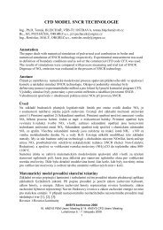
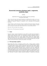
Fig. 2. Design <strong>of</strong> charge <strong>pressure</strong> relief <strong>valve</strong>
Konference ANSYS 2011<br />
2. Charge <strong>pressure</strong> relief <strong>valve</strong> (CPRV)<br />
The function <strong>of</strong> CPRV is <strong>to</strong> maintain charge <strong>pressure</strong> <strong>of</strong> the closed hydrostatic system at a designated level<br />
above case <strong>pressure</strong> (Sauer-Danfoss, 2011). The CPRV is a direct acting poppet <strong>valve</strong> (Fig. 2). It opens and<br />
discharges fluid <strong>to</strong> the pump case when <strong>pressure</strong> exceeds the designated level, p charge , at a channel called gallery.<br />
The <strong>valve</strong> poppet has a cone which acts against a seat created in the pump end cap (Fig. 2). The poppet guiding<br />
is provided by a guide designed in the nut. The 2 springs provide force which acts in direction <strong>to</strong> close the <strong>valve</strong>.<br />
Pretension <strong>of</strong> one spring can be adjusted by a bolt <strong>to</strong> reach desired level <strong>of</strong> the cracking <strong>pressure</strong>. The pretension<br />
force can be calculated from equation:<br />
( ) , (1)<br />
where and radii are evident from Fig. 2.<br />
As the poppet moves, the spring force corresponds <strong>to</strong> equation:<br />
where is spring <strong>rate</strong> and is poppet stroke.<br />
, (2)<br />
3. CFD model<br />
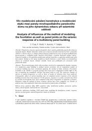
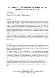
As mentioned above, the <strong>steady</strong> <strong>state</strong> <strong>approach</strong> is used here. The CFD models (Fig. 3) are prepared for 3 poppet<br />
strokes (0.5 mm, 1.5 mm and 3 mm). There is used combination <strong>of</strong> hexahedral, tetrahedral and wedge mesh<br />
types created using ANSYS ICEM CFD.<br />
The CFD analysis is performed in ANSYS Fluent.<br />
Material properties <strong>of</strong> hydraulic oil Shell Tellus 46 are used. The fluid is assumed as incompressible. Based on<br />
previous investigation, experience and comparison with testing, laminar model is chosen in this specific case.<br />
Pressure outlet boundary condition is applied <strong>to</strong> the pump housing passage. The <strong>pressure</strong><br />
constant for all the calculated cases.<br />
Velocity inlet boundary condition is experienced as suitable and stable for this task. Inlet velocity and flow <strong>rate</strong><br />
are related <strong>to</strong> each other by simple relation:<br />
, (3)<br />
where is inlet flow <strong>rate</strong>, is inlet velocity magnitude and is inlet area. The velocity magnitude (flow<br />
<strong>rate</strong> respectively) is ramped <strong>to</strong> several values for each the stroke model. At least, 3 discrete velocity magnitudes<br />
are needed for each the stroke <strong>to</strong> be able approximate results by quadratic function.<br />
As a result from each the CFD <strong>calculation</strong> is:<br />
<strong>pressure</strong> at inlet ( ),<br />
flow force induced by oil <strong>to</strong> the poppet ( ).<br />
is<br />
For reference, <strong>pressure</strong> con<strong>to</strong>urs and streamlines in region <strong>of</strong> control passage are shown in Fig. 4 for 1 mm<br />
poppet stroke and 70 lmin -1 flow <strong>rate</strong> case.
TechS<strong>of</strong>t Engineering & SVS FEM<br />
poppet modeled at 3 stroke<br />
positions<br />
detail <strong>of</strong> hexahedral mesh<br />
in control passage area<br />
<strong>pressure</strong> outlet (p case)<br />
velocity inlet<br />
Fig. 3. CFD model<br />
limits are set manually<br />
Fig. 4. Pressure con<strong>to</strong>urs and streamlines in control passage region<br />
(1 mm stroke, 70 lmin -1 flow)
Konference ANSYS 2011<br />
4. Post-processing<br />
The post-processing plays big role in this task. We have data from 9 CFD <strong>calculation</strong>s (3 strokes × 3 flow <strong>rate</strong>s<br />
per each stroke = 9 <strong>calculation</strong>s) in this specific example. Therefore further data processing in a spreadsheet or<br />
other suitable <strong>to</strong>ol is needed.<br />
The input and output values can be collected in<strong>to</strong> a table form for further processing. One table proposal is<br />
following:<br />
stroke flow <strong>rate</strong> <strong>pressure</strong> drop flow force<br />
Tab. 1. Proposed table for collection <strong>of</strong> CFD inputs and outputs<br />
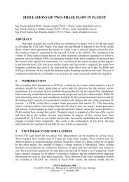
The visualization <strong>of</strong> data points can be seen in Fig. 5. The triangle points in graph C represent dependency <strong>of</strong> the<br />
<strong>pressure</strong> drop on flow <strong>rate</strong>. The different colors relate <strong>to</strong> different poppet strokes. Similarly, the square points in<br />
graph B represent dependency <strong>of</strong> the flow force on flow <strong>rate</strong>.<br />
The data points can be approximated by quadratic polynomial trendlines (continuous colored lines in graphs B<br />
and C) for each the stroke value. The flow force at constant stroke can be then written in form:<br />
where , , and<br />
, (4)<br />
are polynomial coefficients obtained from the spreadsheet trendline properties.<br />
It is obvious the flow force has <strong>to</strong> be in balance with the spring force (2) at each the point <strong>of</strong> final <strong>pressure</strong> <strong>rise</strong><br />
<strong>rate</strong> characteristic. Therefore we can write:<br />
Solution <strong>of</strong> this quadratic equation is:<br />
( ) (5)<br />
√ ( )<br />
, (6)<br />
where the sign plus or minus is chosen in way <strong>to</strong> obtain physically correct result. So, using (6) we get flow <strong>rate</strong><br />
at which there is balance between flow force and spring force at constant stroke (compare graphs A and B in Fig.<br />
5 <strong>to</strong> see balance between spring force and flow force for each the stroke) .
TechS<strong>of</strong>t Engineering & SVS FEM<br />
C<br />
s 1=const.<br />
p s1<br />
p cr<br />
q s1<br />
A<br />
B<br />
s 1=const.<br />
s 1<br />
Fig. 5. Visualisation <strong>of</strong> the <strong>pressure</strong> <strong>rise</strong> <strong>rate</strong> characteristic design<br />
Similarly <strong>to</strong> the flow forces approximation, we can also approximate the <strong>pressure</strong> drop data points using<br />
quadratic polynomial trendlines in form:<br />
, (7)<br />
where the polynomial coefficients , , and are obtained again from the spreadsheet trendline properties. If we<br />
use the calculated flow <strong>rate</strong> from (6), we obtain corresponding <strong>pressure</strong> drop:<br />
, (8)<br />
This procedure is repeated for all the 3 strokes so we obtain the flow <strong>rate</strong> and <strong>pressure</strong> drop pairs:<br />
[ ] [ ] [ ] (9)<br />
plus we have the additional point [<br />
] The final <strong>pressure</strong> <strong>rise</strong> <strong>rate</strong> characteristic can be designed from<br />
those points – see red line in graph C in Fig. 5.<br />
5. Comparison with measurement<br />
A simplified hydraulic scheme used for measurement <strong>of</strong> the CPRV is shown in Fig. 6a. An auxiliary pump H<br />
provides oil <strong>to</strong> the testing device. The throttle <strong>valve</strong> TV is fully open so the <strong>pressure</strong> indicated by the gauge G1 is<br />
small in comparison with the cracking <strong>pressure</strong> <strong>of</strong> the tested CPRV. As the TV restricts flow area, the load <strong>of</strong>
Konference ANSYS 2011<br />
CPRV increases and it starts <strong>to</strong> ope<strong>rate</strong>. Pressure before CPRV (G1) and behind it (G2) is recorded <strong>to</strong>gether with<br />
flow <strong>rate</strong> (Q). Note the measurement process should be sufficiently slow <strong>to</strong> avoid dynamic effects <strong>of</strong> the system.<br />
It is possible <strong>to</strong> perform measurement <strong>of</strong> the CPRV installed in a simple test block or installed in the pump end<br />
cap. The measured <strong>valve</strong> performance with the one calculated by CFD are shown in Fig. 6b for comparison.<br />
G1<br />
G2<br />
CPRV<br />
TV<br />
Q<br />
H<br />
a<br />
b<br />
Fig. 6. Measurement hydraulic scheme (a) and comparison CFD with measurement (b)<br />
6. Conclusion<br />
The design <strong>of</strong> <strong>pressure</strong> <strong>rise</strong> <strong>rate</strong> characteristic <strong>of</strong> charge <strong>pressure</strong> relief <strong>valve</strong> using <strong>steady</strong> <strong>state</strong> CFD simulation is<br />
shown in the article. The model is prepared for 3 constant strokes. Minimally 3 different flow <strong>rate</strong> conditions<br />
needs <strong>to</strong> be calculated for each the stroke due <strong>to</strong> possibility <strong>of</strong> data approximation by quadratic polynomial<br />
functions. Both <strong>pressure</strong> drop and flow force functions are approximated in relation <strong>to</strong> flow <strong>rate</strong>. The final<br />
<strong>pressure</strong> <strong>rise</strong> <strong>rate</strong> characteristic <strong>of</strong> the <strong>valve</strong> is found using condition <strong>of</strong> equilibrium <strong>of</strong> flow force and spring<br />
force at each the specific stroke.<br />
Because <strong>of</strong> computing only a few <strong>steady</strong> <strong>state</strong> cases, the proposed method saves computing time as well as effort<br />
<strong>to</strong> set up the analysis in comparison <strong>to</strong> transient CFD computation.<br />
Another advantage is the effect <strong>of</strong> the cracking <strong>pressure</strong> or spring <strong>rate</strong> change is re-calculated immediately in the<br />
spreadsheet without any additional CFD <strong>calculation</strong> requirement.<br />
7. Bibliography<br />
1. “H1 Axial Pis<strong>to</strong>n Pumps Single and Tandem”, Basic Information, Sauer-Danfoss, 11062168-Rev BB-Apr<br />
2011.<br />
2. Imre M., Kriššák P., Rahmfeld R., Zavadinka P., “Porovnanie simulačných a meraných výsledkov<br />
škrtiaceho ventila”, Hydraulika a pneumatika, 1-2/2010, ISSN 1335-5171.